Journal of Financial Planning: November 2013
Executive Summary
- This study examines the asset location issue by answering the question of whether it is better to locate stocks in taxable accounts and bonds in tax-deferred accounts like a traditional IRA to the extent possible, while attaining the investor’s desired asset allocation, or vice versa?
- Two groups of studies have examined this issue. The first uses the traditional approach to calculate an investor’s asset allocation and generally has concluded that the optimal asset location decision depends upon specific assumptions about returns and tax rates. The second group uses the after-tax approach to calculate an investor’s asset allocation and generally has concluded that the optimal asset location decision is to locate stocks in taxable accounts and bonds in retirement accounts to the extent possible while attaining the target asset allocation.
- An after-tax mean-variance optimization framework is used to examine the asset location issue. Within this framework it is shown that stocks and bonds held in a taxable account and a tax-deferred or tax-exempt account are effectively four different assets. The asset location and asset location decisions are jointly made.
- This paper concludes by indicating that except in rare cases, investors should hold stocks in taxable accounts and bonds in retirement accounts.
William Reichenstein, Ph.D., CFA, holds the Pat and Thomas R. Powers Chair in Investment Management at Baylor University. He also is head of research at Social Security Solutions Inc. and Retiree Income Inc.
Email HERE.
William Meyer is founder and CEO of Social Security Solutions Inc., a developer of software to help advisers make Social Security claiming decisions. He also is founder and CEO of Retiree Income Inc., a developer of software that calculates investors’ after-tax asset allocation and provides asset location advice. Email HERE.
Two groups of studies have examined whether, everything else the same, it is better to locate stocks in taxable accounts and bonds in tax-deferred accounts (for example, traditional IRAs), to the extent possible, while attaining the investor’s desired asset allocation. The first group includes studies by Daryanani (2004), Daryanani and Cordaro (2005), Jaconetti (2007), Kitces (2013), Shoven (1999), Shoven and Sialm (1998), and Trout (2013). These studies assume constant rates of return on stocks and bonds and ask whether the ending after-tax wealth is larger when stocks are held in a tax-deferred account like a traditional IRA, and bonds are held in a taxable account or vice versa.
These studies use the traditional approach to calculate an investor’s asset allocation. These approaches consider the impact of the asset location decision on ending after-tax wealth (that is, they consider after-tax returns), but they do not recognize that the asset location decision also affects the after-tax risk borne by investors. These studies generally conclude that the optimal asset location decision depends upon specific assumptions about returns and tax rates.
A second group of studies include Dammon, Spatt, and Zhang (2004), Horan (2007a, 2007b), Horan and Al Zaman (2008), Reichenstein (2001a, 2001b, 2006, 2007a, 2007b, 2008), Reichenstein and Jennings (2003), and Reichenstein, Horan, and Jennings (2012). These studies use an after-tax asset allocation framework where taxes are considered when calculating an investor’s current asset allocation. These researchers also recognize that the asset location decision affects the after-tax risk borne by the investor. Financial planners all agree, of course, that investors are concerned about returns and risk. When it is shown that the asset location decision also impacts after-tax risk, it is clear that the second approach should be used to address the asset location decision.
A representative example from the first group of studies is presented that will show such studies’ shortcomings. Examples using an after-tax mean-variance framework that avoids these shortcomings is then presented.
Tax-Deferred Accounts as Partnerships
As described in Horan (2005, 2007a, 2007b), Horan and Al Zaman (2008), Reichenstein (2001a, 2001b, 2006, 2007a, 2007b, 2008), Reichenstein and Jennings (2003), and Reichenstein et al. (2012), the best way to view a tax-deferred account (TDA) is as a partnership. The investor effectively owns (1-t) of the TDA’s principal, where t is the marginal tax rate when the funds are withdrawn in retirement, while the government effectively owns the remaining t of the principal. The investor, as majority partner, can move funds among asset classes as he or she chooses. But every time the investor withdraws funds from the TDA, the government as minority partner, takes t of that distribution as taxes.
Assume an investor will have a 30 percent marginal tax rate in retirement. It is instructive to compare the after-tax future values of $1 of pre-tax funds in a tax-deferred account to $0.70 of after-tax funds in a tax-exempt account (TEA) like a Roth IRA. To hold everything else constant, assume these funds are invested in the same asset. It could be a stock or bond, and the length of the investment horizon could be short or long.
Assume the underlying investment earns a pre-tax return of r percent and will be withdrawn n years hence. The $1 of pre-tax funds in the tax-deferred account is worth $1(1+r)n before taxes in n years. After withdrawal, it is worth $1(1+r)n(1 – 0.3) or $0.70(1+r)n after taxes. Similarly, after withdrawal n years hence, the tax-exempt account is worth $0.70(1+r)n after taxes.
When calculating this investor’s asset allocation, the $1 of pre-tax funds in a TDA should be considered equivalent to $0.70 of after-tax funds in a TEA. To continue with the partnership concept, it is useful to separate the $1 of pre-tax funds in the TDA into $0.70 of the investor’s after-tax funds plus $0.30, which is the government’s share of the current principal.
This partnership concept has implications for the calculation of the investor’s asset allocation. Suppose this investor has $1 of pre-tax funds in a TDA held in bonds, $0.70 of after-tax funds in a TEA held in stocks. The traditional approach to calculating her asset allocation would say she has a 59 percent bonds/41 percent stocks asset allocation. This approach does not recognize the embedded tax liability in the TDA. It does not acknowledge that the investor effectively owns only (1 – t) of the TDA’s pre-tax market value.
In contrast, the after-tax approach to calculating her asset allocation would first convert the $1 of pre-tax funds in the TDA to $0.70 of the investor’s after-tax dollar. It would then calculate her after-tax asset allocation using after-tax values. In this approach, she has $0.70 of after-tax funds in bonds held in a TDA, and $0.70 of after-tax funds in stocks held in a TEA for an after-tax asset allocation of 50 percent bonds/50 percent stocks.
The after-tax asset allocation compares after-tax funds to after-tax funds, while the traditional approach fails to distinguish between pre-tax funds and after-tax funds. Because the traditional approach is tax oblivious, it implicitly assumes the investor’s tax rate in retirement will be zero percent. Although an investor’s retirement tax rate may be unknown, for most investors and virtually all financial planning clients, it is easy to improve upon the traditional approach’s implicit assumption of a zero percent tax rate. Simply put, it is better to estimate the marginal tax rate in retirement and calculate an individual investor’s after-tax asset allocation that is approximately right than to implicitly assume the client will have a zero percent tax rate in retirement and thus calculate a traditional asset allocation that is precisely wrong. As this paper highlights, the first group of studies uses the traditional approach to calculating the asset allocation, failing to distinguish between pre-tax funds and after-tax funds.
After-Tax Risk and Returns across Savings Vehicles
The first group of studies considers the impact of the asset location decision on the investors’ after-tax returns, but these analyses do not explicitly recognize that the asset location decision also affects the after-tax risk borne by the investor.
To conform with an example from a recent study, assume that the ordinary income tax rate is 30 percent, the long-term capital gain tax rate is 15 percent, and pre-tax returns on bonds and stocks are 5 percent and 8 percent, respectively, with all stock returns in the form of capital gains that are realized in one year and one day so that the long-term capital gain tax rate applies.
The tax-exempt account begins with $1 of after-tax funds. After withdrawal in n years, the after-tax bond value is $1(1.05)n. The investor’s after-tax value grows tax free from $1 today to $1(1.05)n after withdrawal, where 5 percent is the bond’s pre-tax rate of return. Similarly, after withdrawal in n years the after-tax stock value is $1(1.08)n. The after-tax value grows tax free at the stock pre-tax rate of return. When held in a TEA, the investor receives 100 percent of pre-tax returns and bears 100 percent of pre-tax risk whether the underlying asset is bonds or stocks.
The tax-deferred account begins with $1 of pre-tax funds, which is best viewed as $0.70 of the investor’s after-tax funds with the government owning the remaining $0.30. Before withdrawal in n years, the pre-tax bond value is $1(1.05)n. After withdrawal, the after-tax value is $0.70(1.05)n. The investor’s after-tax value grows tax free from $0.70 today to $0.70(1.05)n after withdrawal. Similarly, before withdrawal in n years, the pre-tax stock value is $1(1.08)n. After withdrawal, the after-tax value is $0.70(1.08)n. Whether the underlying asset is bonds or stocks, the investor’s after-tax value grows from $0.70 today to $0.70(1+r)n at withdrawal, where r is the underlying asset’s pre-tax rate of return. Therefore, when held in a TDA, the investor receives 100 percent of pre-tax returns and bears 100 percent of pre-tax risk whether the underlying asset is bonds or stocks.
To be consistent with examples in the first group of studies, assume the taxable account begins with $1 of after-tax funds; that is, the market value and cost basis are each $1. The after-tax value of the bond grows from $1 today to $1(1 + 0.05(1 – 0.3))n or to $1(1.035)n at withdrawal.¹ Similarly, the after-tax value of the stock grows from $1 today to $1(1 + 0.08(1 – 0.15))n or to $1(1.068)n at withdrawal. The investor gets 70 percent of the pre-tax bond return and 85 percent of the pre-tax stock return. The risk borne by the investor is examined next.
Assume pre-tax returns on stocks are –7 percent, 8 percent, and 23 percent in a three-year period. The pre-tax mean return is 8 percent and pre-tax standard deviation is 15 percent. The 8 percent and 23 percent pre-tax returns become 6.8 percent and 19.55 percent after taxes. Assuming the 7 percent loss can be used to offset long-term gains, this loss becomes a –5.95 percent return after taxes. With this assumption, when stocks are held in a taxable account the investor’s returns are –5.95 percent, 6.8 percent, and 19.55 percent. The investor receives 85 percent of pre-tax returns and bears 85 percent of pre-tax risk. Similarly, since the government takes some of the bonds return, it also bears some of bond risk. The investor receives 70 percent of the pre-tax bond returns and bears 70 percent of the pre-tax bond risk. Reichenstein (2008) expanded this type of analysis to include dividend paying stocks.
Reichenstein (2001a, 2008), Reichenstein et al. (2012), and Reichenstein and Jennings (2003) considered investors with different stock management practices including (1) day traders who realize all returns each year as short-term gains that are taxed as ordinary income, (2) active investors who realize all gains after one year and one day, (3) passive investors who let gains grow unharvested until realized in n years, and (4) exempt investors who either sell the stock after receiving the step-up in basis at death or donate the appreciated asset to a qualified charity. Except for the extreme examples of non-dividend paying stocks held by a day trader or an exempt investor, the investor bears less than 100 percent of the risk on the asset held in a taxable account. So, the conclusion that the investor does not bear all of the risk of assets held in taxable accounts remains valid for all but a few investors.
Brunel (2001, 2004) expanded the asset location issue to include assets held in trusts and other savings vehicles.
Example from Recent Literature
The first group of studies examined whether, everything else the same, it is better to locate stocks in taxable accounts and bonds in TDAs, or vice versa. For example, Daryanani and Cordaro (2005) calculated the after-tax ending wealth to two asset location strategies assuming a 30-year investment horizon, 30 percent ordinary income tax bracket, 15 percent capital gain tax bracket, 5 percent bond returns, and 8 percent stock returns in the form of capital gains that are realized each year (technically, in one year and one day). The after-tax ending wealth values for initial investments of $500,000 of pre-tax funds in TDAs and $500,000 of after-tax funds in taxable accounts are as follows:
Strategy 1: stocks in tax-deferred account
Bonds in taxable accounts: $500,000 (1 + .05(1–0.3))30 = $1,403,397
Stocks in TDA: $500,000 (1.08)30 (1–0.3) = $3,521,930
Total: $4,925,327
Strategy 2: bonds in tax-deferred account
Stocks in taxable accounts: $500,000 (1 + .08(1–0.15))30 = $3,598,385
Bonds in TDA: $500,000 (1.05)30 (1–0.3) = $1,512,680
Total: $5,111,065
Based on the assumptions, Daryanani and Cordaro (2005) concluded that stocks should be located in taxable accounts and bonds in TDAs. However, the optimal asset location in this framework depends upon the specific assumptions. Daryanani and Cordaro noted that the opposite asset location is optimal if any one of the following change, everything else held constant: (1) the capital gain tax rate is 20 percent; (2) stocks earn 10 percent a year; (3) horizon is 40 years; or (4) the ordinary income tax rate is 25 percent. As they stated, “Clearly, the results are dependent on the input assumptions.” (p. 45)
The objective of asset location studies is to determine which strategy is better holding everything else constant. It appears that Daryanani and Cordaro (2005) were thinking along the following lines (material in parentheses was added by the authors):
- Investors should approach the asset location decision as a two-step process. First, determine the target asset allocation (as traditionally defined). Second, make the asset location decision.
- Because the (traditionally-defined) asset allocation decision is the same for both asset locations, the investor’s portfolio risk is the same regardless of his asset location decision.
- With portfolio risk held constant, an investor can compare the ending wealth values, and select the asset location decision that maximizes ending wealth. This additional ending wealth is a pure gain attributable to the asset location decision.
With this framework in mind, the next step is to examine the shortcomings of this approach when the after-tax approach of calculating an investor’s asset allocation is substituted. Daryanani and Cordaro (2005) did not hold the investor’s initial after-tax asset allocation constant. Rather, the asset location decision affects the initial after-tax asset allocation.
In Strategy 1 noted earlier, the investor begins with $500,000 of after-tax funds in bonds and $350,000 of after-tax funds in stocks for a 59 percent bonds/41 percent stocks after-tax asset allocation. The “stocks in tax-deferred account” calculation of $500,000(1 – 0.3)(1.08)30 simplifies to $350,000(1.08)30. This shows that the $500,000 of pre-tax funds in the TDA is best viewed as $350,000 of the investor’s after-tax funds with the government owning the remaining $150,000.
In Strategy 2, the investor begins with $350,000 of after-tax funds in bonds held in TDAs and $500,000 of after-tax funds in stocks held in taxable accounts for an after-tax asset allocation of 41 percent bonds/59 percent stocks.
These asset location strategies also have different asset allocations at other times. For example, Strategy 1 has an ending asset allocation whether calculated using the traditional approach or after-tax approach of 28 percent bonds/72 percent stocks,2 while Strategy 2 has an ending asset allocation of 30 percent bonds/70 percent stocks.
Additionally, these asset location strategies provide the investor with different initial after-tax returns and after-tax risks. Strategy 1 has an initial after-tax expected return of 5.35 percent,3 and Strategy 2 has an initial after-tax return of 6.06 percent. Assuming pre-tax standard deviations of 6 percent for bonds, 15 percent for stocks, and a correlation coefficient of 0.2, Strategy 1 has an initial after-tax standard deviation of 7.10 percent, and Strategy 2 has an initial standard deviation of 8.35 percent.4
These asset location strategies also have different after-tax returns and after-tax risks at other times. For example, Strategy 1 has an ending after-tax expected return of 6.72 percent and after-tax risk of 11.03 percent, while Strategy 2 has ending after-tax returns and risk of 6.27 percent and 9.49 percent.
When viewed from the perspective of an after-tax asset allocation, these studies do not change the asset location decision, while holding everything else constant. Differences in the ending wealth from the two strategies are due to differences in asset location decisions, after-tax asset allocations, and after-tax returns and risks. Moreover, as will be shown, the two-step procedure of first determining the asset allocation and then determining the asset location is inappropriate.
Mean-Variance Optimization
Because the asset location decision affects the portfolio’s after-tax risk and after-tax returns, the mean-variance framework provides a better approach to address the asset location decision. Reichenstein (2001a, 2008), Reichenstein and Jennings (2003), Horan and Al Zaman (2008), and Reichenstein et al. (2012) each provide frameworks built on the key ideas in this study.
The discussion continues with the earlier mentioned assumptions from Daryanari and Cordaro (2005). The utility function is U = ER – 0.005RAσ2, where ER denotes after-tax expected return, σ2 is the after-tax variance, and RA is the level of risk aversion.5 Utility, U, also denotes the risk-free return that would provide the same level of utility as the portfolio.
To illustrate the problems with the first group of studies, it is instructive to begin with a traditional mean-variance optimization. Table 1 presents these results. The risk aversion level is set at 3.175 because this is the level that produces the 50 percent bonds/50 percent stocks asset allocation as measured using the traditional approach. Sharpe (1990) estimated that the societal average risk tolerance has been 50 for the post-1926 period, which corresponds to a risk aversion level of 4.
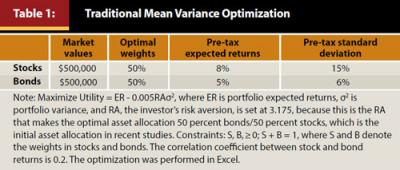
Due to the assumed historically low equity risk premium of 3 percent, it takes someone with below-average risk aversion to attain the 50 percent/50 percent asset mix. Because the traditional approach ignores taxes, the optimization only considers pre-tax returns and pre-tax risks. The model does not recognize that the government bears some risk on the assets held in taxable accounts. Moreover, the traditional approach does not consider the embedded tax liability in the tax-deferred account.
Table 2 presents the after-tax mean variance optimization. The first step to performing an after-tax optimization is to calculate the size of the investor’s after-tax portfolio. The investor’s after-tax portfolio contains $350,000 of after-tax funds in tax-deferred accounts and $500,000 of after-tax funds in taxable accounts for a total of $850,000. The second step is to insert the after-tax returns and risk for both bonds and stocks when held in a TDA and a taxable account, respectively. The after-tax returns and risk for bonds and stocks when held in a TDA are the same as their pre-tax values. When held in taxable accounts, the after-tax bond return is 3.5 percent and after-tax risk is 4.2 percent. For the stock investor who realizes gains at the end of each year, the after-tax stock return is 6.8 percent and after-tax risk is 12.75 percent.Even though there are only two assets, there effectively are four “assets” in the optimization, because bonds and stocks are different assets when held in a TDA and a taxable account.
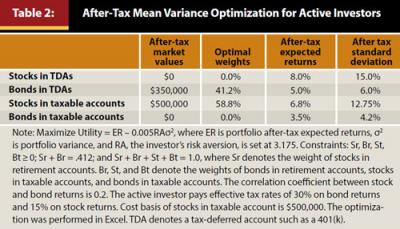
In Table 2, the optimal after-tax asset allocation is 41.2 percent bonds/58.8 percent stocks. The optimal asset location is to hold bonds in the TDA and stocks in the taxable account. Unlike the traditional optimization approach, the after-tax optimization is not silent on the issue of asset location. The stock allocation is heavier in the after-tax optimization than in the traditional optimization. Because the investor only bears 85 percent of risks associated with stocks when held in taxable account, the investor can bear a heavier stock allocation for a given level of risk aversion.
Table 3 presents other results from this after-tax mean-variance framework. Portfolio 1 summarizes the base case portfolio for a more typical risk aversion level of 3.85. The optimal after-tax asset allocation is 41.2 percent bonds and 58.8 percent stocks. The optimal asset location is to hold bonds in retirement accounts (TDAs or TEAs) and stocks in taxable accounts. The after-tax expected return is 6.06 percent. The after-tax standard deviation is 8.35 percent, and the maximum utility is 4.72 percent.
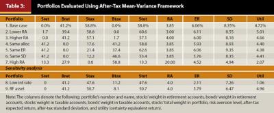
Portfolios 2 and 3 present the results for, respectively, lower and higher levels of risk aversion than in the base case. In Portfolio 2, the investor has a lower risk aversion of 3, and the investor holds stocks and bonds in the retirement account, but she only holds stocks in the taxable account. In Portfolio 3 the investor has a higher risk aversion of 4, and holds stocks and bonds in the retirement account, but she only holds stocks in the taxable account. It is important to note that an investor should never hold bonds and stock in both retirement accounts and taxable accounts. These results emphasize that the optimal asset location decision is to locate bonds in retirement accounts and stocks in taxable accounts to the extent possible, while attaining the target asset allocation.
Portfolio 4 presents the results if the investor has the same after-tax asset allocation as in the base case, but a different asset location decision. Portfolio 4 holds only stocks in retirement accounts but a combination of stocks and bonds in the taxable account to attain the 41.2 percent/58.8 percent bonds/stocks asset allocation. The utility of this portfolio is 0.32 percent lower than the utility in the base case portfolio. Thus, the same asset allocation but wrong asset location decision costs this investor 0.32 percent of certainty equivalent return.
Portfolio 5 was constructed to have the same expected return as the base case portfolio, but the wrong asset location. By holding only stocks in the retirement account and holding stocks and bonds in the taxable account, Portfolio 5 provides the same expected return as Portfolio 1, but it has a higher risk. Compared to Portfolio 1, Portfolio 5 costs this investor 0.34 percent of certainty equivalent return.
Portfolio 6 was constructed to have the same standard deviation as the base case portfolio, but the wrong asset location. Portfolio 1 provides a higher expected return for the same level of risk than is possible with Portfolio 6. Compared to Portfolio 1, Portfolio 6 costs this investor 0.31 percent of certainty equivalent return.
Results from these analyses suggest that the usual asset location advice henceforth should be the following: An investor should locate bonds in retirement accounts (TDAs and TEAs) and stocks in taxable accounts to the extent possible, while attaining the target asset allocation. This advice holds for most, but not all, risk aversion levels. Portfolio 7 assumes a risk aversion level of 20. At this level or higher, the usual location advice does not prevail. Rather, this investor should hold bonds and stock in the retirement account, but only bonds in the taxable account. Based on this unusual asset location advice, it is important to consider the implications of a risk aversion level of 20 compared to those assumed in Portfolios 1 through 6.
Sensitivity Analysis
Recent asset location studies ask an excellent question: Given today’s historically low interest rates, should individual investors still locate bonds in retirement accounts and stocks in taxable accounts? Portfolio 8 (see Table 3) examines this issue for an investor with an average risk aversion level of 4. It presents the results when expected returns on bonds and stocks are lowered to 1 percent and 4 percent, respectively, thus maintaining the 3 percent equity risk premium. The standard deviations on bonds and stocks are the same as in the base case. As the results for Portfolio 9 show, the usual asset location advice prevails for investors with average risk aversion. However, for investors with above-average risk aversion the usual advice does not prevail. At risk aversion levels between 4.08 and 4.35, stocks and bonds are held in both retirement accounts and taxable accounts. At risk aversion levels of 4.44 or higher, stocks and bonds are held in retirement accounts, while only bonds are held in taxable accounts.
To further consider the implications of today’s low yields, other risk and return assumptions were examined. As is well known, the mean-variance optimization framework does not address the length of the investment horizon. If the horizon is intermediate term or long term, then today’s bond returns would likely be set at today’s intermediate-term or long-term yield on high-grade bonds. These yields are higher than the 1 percent assumed in Portfolio 8.
If expected returns are set at 2 percent for bonds and 5 percent for stocks, while standard deviations are set at 6 percent and 15 percent, then the usual asset location advice prevails at risk aversion levels of 7.47 or lower. If the horizon is shorter term, then the standard deviation of bonds would likely be lower.
If expected returns are maintained at 1 percent for bonds and 4 percent for stocks, while standard deviations are set at 3 percent and 15 percent, then the usual asset location advice prevails at risk aversion levels of 13.2 or lower. Consequently, it appears that, even given today’s low interest rates, the usual asset allocation recommendation prevails for most investors. Nevertheless, it is important to note that sufficiently low interest rates could affect the usual asset location advice, especially for investors with above-average risk aversion.
Finally, Portfolio 9 presents the results from a mean-variance optimization when the fixed-income asset is a risk-free asset. This portfolio repeats the base case assumptions, but the standard deviation for bonds is set at 0 percent. In this case, the usual asset location advice prevails. Moreover, various combinations of returns and risk were tested, and as long as the risk of bonds is set at 0 percent the usual asset allocation advice prevails.
Conclusions
This study has revealed that the traditional approach to calculating an individual’s asset allocation does not adjust the TDA’s market value for the embedded tax liability. Furthermore, it does not recognize that the government takes some of the return and bears some risk of assets held in taxable account. Therefore, the same asset, whether stock or bond, is effectively a different asset when held in a TDA or taxable account.
Results from this analysis indicate that the usual asset location advice is for an individual investor to locate stocks in taxable accounts and bonds in retirement accounts (TDAs and TEAs) to the extent possible, while attaining the optimal asset allocation. Even with today’s historically low interest rates, this usual asset location advice prevails for most investors. However, exceptionally low yields can reverse the usual asset location advice, especially for individuals with above-average risk aversion. Finally, the usual asset location advice prevails for investors who select a risk-free asset for the fixed-income portion of their portfolios.
Endnotes
- If the taxable bond offers a 5 percent yield, then a tax-exempt bond may offer a yield of 3.5 percent. In this case, this tax-exempt bond has an implicit tax rate of 30 percent. Properly viewed, the tax-exempt investor is paying a 30 percent implicit tax rate.
- [$1,403,397/$4,925,327]
- [3.5 percent ($500,000/$850,000) + 8 percent ($350,000/$850,000)]
- For Strategy 1, the initial standard deviation is [($500/850)² (.042)2 + ($350/850)2 (.15)2 + 2($500/850) ($350/$850) (.042) (.15) .2]1/2, where .042 is .06(1-.3) or the product of 6 percent pre-tax risk and (1 minus the 30 percent tax rate). Strategy 2’s initial standard deviation is [($500/850)2 (.1275)2 + ($350/850)2 (.06)2 + 2($500/850) ($350/$850) (.1275) (.06) .2]1/2, where .1275 is the product of 15 percent pre-tax risk and (1 minus 15 percent capital gain tax rate).
- Sharpe (1990) uses an equivalent utility function: U = ER – σ2/RT, where RT is the level of risk tolerance. When returns are expressed as integers (e.g., 8 percent) as in this study then RA = 200/RT. When returns are expressed as decimals (e.g., 0.08) then U = ER – 0.5RA σ2 = ER - σ2RT and RA = 2/RT. Nanigian (2011) discusses the rationale for using a utility function.
References
Brunel, Jean. 2004. “The Tax Efficient Portfolio.” In The Investment Think Tank, edited by Harold Evensky and Deena Katz, 5–16. Princeton, New Jersey: Bloomberg Press.
Brunel, Jean. 2001. “Asset Location—The Critical Variable: A Case Study.” Journal of Wealth Management 4 (1): 27–43.
Dammon, Robert M., Chester S. Spatt, and Harold H. Zhang. 2004. “Optimal Asset Location and Allocation with Taxable and Tax—Deferred Investing.” Journal of Finance 59 (3): 999–1037.
Daryanani, Gobind. 2004. “A Different Approach to Asset Location.” In The Investment Think Tank, edited by Harold Evensky and Deena Katz, 125–148. Princeton, New Jersey: Bloomberg Press.
Daryanani, Gobind, and Chris Cordaro. 2005. “Asset Location: A Generic Framework for Maximizing After-Tax Wealth.” Journal of Financial Planning (18) 1: 44–54.
Horan, Stephen M. 2005. Tax-Advantaged Savings Accounts and Tax-Efficient Wealth Accumulation. Charlottesville, Virginia: Research Foundation of CFA Institute.
Horan, Stephen M. 2007a. “An Alternative Approach to After-Tax Valuation.” Financial Services Review (16) 3: 167–182.
Horan, Stephen M. 2007b. “Applying After-Tax Asset Allocation.” Journal of Wealth Management (10) 2: 84–93.
Horan, Stephen M., and Ashraf Al Zaman. 2008. “Tax-Adjusted Portfolio Optimization and Asset Location: Extensions and Synthesis.” Journal of Wealth Management (11) 3: 56–73.
Jaconetti, Colleen M. 2007. “Asset Location for Taxable Investors.” Vanguard Investment Counseling and Research. personal.vanguard.com/pdf/s556.pdf
Kitces, Michael. 2013. “Asset Location: The New Wealth Management Value-Add for Optimal Portfolio Design?” The Nerd’s Eye View blog, March 6.
Nanigian, David. 2011. “A More Informative Measure of Active Fund Performance.” Journal of Financial Planning (24) 11: 54–60.
Reichenstein, William. 2001a. “Asset Allocation and Asset Location Decisions Revisited.” Journal of Wealth Management (4) 1: 16–26.
Reichenstein, William. 2001b. “Rethinking the Family’s Asset Allocation.” Journal of Financial Planning (14) 5: 102–109.
Reichenstein, William. 2006. “After-Tax Asset Allocation.” Financial Analysts Journal (62) 4: 14–19.
Reichenstein, William. 2007a. “Calculating After-Tax Asset Allocation is Key to Determining Risk, Returns, and Asset Location.” Journal of Financial Planning (20) 7: 44–53.
Reichenstein, William. 2007b. “Implications of Principal, Risk, and Returns Sharing across Savings Vehicles.” Financial Services Review (16) 1: 1–17.
Reichenstein, William. 2008. In the Presence of Taxes: Applications of After-tax Asset Valuations. Washington, DC: FPA Press.
Reichenstein, William, Stephen H. Horan, and William W. Jennings. 2012. “Perspectives: Two Key Concepts for Wealth Management and Beyond.” Financial Analysts Journal (68) 1: 14–22.
Reichenstein, William, and William W. Jennings. 2003. Integrating Investments and the Tax Code. New York, New York: John Wiley and Sons Inc.
Sharpe, William F. 1990. “Asset Allocation.” In Managing Investment Portfolios: A Dynamic Process, 2nd edition edited by John L. Maginn and Donald L. Tuttle. New York, New York: Warren, Gorham, and Lamont.
Shoven, John B. 1999. “The Location and Allocation of Assets in Pension and Conventional Savings Accounts.” Working Paper No. 7007, NBER, March. www.nber.org/papers/w7007.
Shoven, John B., and Clemens Sialm. 1998. “Long Run Asset Allocation for Retirement Savings.” Journal of Wealth Management (1) 2: 13–26.
Trout, R. Kevin. 2013. “An In-Depth Look at the Tax Consequences of Asset Location.” AAII Journal (35) 3: 26–33.
Citation
Reichenstein, William, and William Meyer. 2013. “The Asset Location Decision Revisited.” Journal of Financial Planning 26 (11): 48–55.