Journal of Financial Planning: February 2011
D. Allen Cohen, Ph.D., is a senior analyst at Navigator Wealth Management in McLean, Virginia, where he developed the in-house model described in this article. He is a former U.S. Air Force captain and performed military operations analysis for 35 years. He received his Ph.D. in theoretical physics from Case Institute in Cleveland, Ohio, in 1960.
Executive Summary
- This article presents an innovative approach to projecting intermediate-term statistical market trends, permitting advantageous adaptations of client portfolio allocations. We call this “slow-timing the market.”
- A simple, automatable algorithmic procedure is put forth for identifying bullish and bearish market trends with durations generally greater than primary-trend durations and less than those of secular trends.
- The algorithm uses the trailing 12-month average of the constant, 1901-dollar Standard & Poor’s 500 Composite Stock Price Index to identify intermediate maxima and minima of the market. A trend change takes from two to six months to recognize; however, the shortest such trend over the past 106 years was 9 months, and the longest was 112 months, invariably permitting such trends to be recognized and advantageously leveraged before they change.
- Statistical distributions of the major security-index total returns were derived separately for these intermediate-trend bullish and bearish periods spanning the past century and programmed into a Monte Carlo model to test the efficacy of slow-timing the market.
- Candidate client bullish and bearish portfolio allocation strategies were evaluated using the model.
- The model statistically projects trend durations as well as trend-recognition lag times. The model subsequently statistically projects the behaviors of the portfolio-allocation strategies (month-to-month) in accordance with the then-current market trend as each run is projected forward in time.
- Definite improvements resulted using this approach versus maintaining allocations independent of market trends.
The opinions herein are those of the author. As with any investment approach, legal and financial-planning professionals should be consulted prior to initiating and in association with any action based on the above approach. The author wishes to acknowledge the critical editing support of Drs. Kenneth Cliffer and Lee Cohen. Thank you.
The object of this paper is to present an alternative to the normative financial planning strategy of persistently maintaining existing allocations during recessions and riding the recession out. The portfolios of clients in good financial planning practices generally are broadly diversified and suffer least from recessions like the most recent one. Nevertheless, the challenge for the analytical approach presented here, which was under refinement at the time of the past recession, was to determine whether a better approach could be devised and practiced. The core of the challenge was seen as understanding and representing market bullish and bearish trends. Even though some researchers have questioned the validity of market trends,1 the following trends are generally accepted: secular, multi-year trends, primary, multi-month trends (approximately 20 percent change in a quarter indicates a trend change), and secondary, multi-day trends (rallies, corrections).
In his book, Unexpected Returns2, Ed Easterling defines secular trends in terms of major trend-maxima and trend-minima in the 12-month trailing average of the P/E ratio of the S&P 500 Index over the last century. In that time span there have been four secular bull periods (of 9, 3, 23, and 17 years) and four secular bear periods (of 19, 3, 4, and 15 years). By way of comparison, six U.S. primary bear markets and five U.S. primary bull markets have occurred in the 30 years from 1973 to 2003.3 The shortest primary bear period was one month with three primary bear periods lasting fewer than five months. The point of emphasizing these secular and primary trend durations is to demonstrate that neither type of trend is appropriate in financial planning management for tailoring portfolio allocations to take advantage of market trends.4,5 Secular trends can be too long and primary trends can be too short.
This observation leads to the principal goal of this endeavor: a reasonably simple algorithm that locates intermediate-term maxima and minima of an appropriate market measure indicating bullish and bearish trends with durations affording a practical and advantageous means of tailoring portfolio allocations.
Intermediate Secular Market Trends
In the proposed approach, the selected market measure is the trailing, 12-month average of the constant-dollar (1901) S&P 500 Index, and the trend-change indicator is a change in this average by 3 percentage points within a six-month period. When this happens, the beginning of the new trend is pegged to the month that the trend change began.
The S&P 500 Index was chosen because it has standing in the industry, it has good and readily available price data that date back for more than a century, and it has been well maintained. In Easterling’s use of the P/E ratio, the primary role of earnings appeared to be to cancel out the effects of inflation. Because consumer price index (CPI) data also date back to the beginning of the last century, the S&P 500 Index can be expressed in constant-dollar values. The year 1901 was chosen as the reference date to allow forward-projected real values for all analyses, including historical analyses. The monthly inflation was calculated as the trailing 12-month average of the monthly percentage change in the CPI. The inflation divisor for any given month is the compounded monthly inflation over all the preceding months starting with January 1901.
Note that the analyses can readily be done with available data and an analytical spreadsheet. The threshold of 3 percent change within six months to characterize a trend transition was chosen because the resulting trend periods, as will be illustrated, are of durations that permit practical alterations of portfolio allocations based on the prevailing bullish or bearish trend. Trend-duration statistics are relatively insensitive to small variations in this algorithm. “Slow-timing the market” is here defined as changing from bullish allocations to bearish allocations and vice versa once an intermediate secular trend change has been detected.6 Once the transition criteria are set, no additional human judgment is involved in deciding if and when a trend transition has taken place; this adherence to pre-established criteria helps clients temper emotional influences on their decisions of whether, when, and what to change.
Figure 1 illustrates the results of defining intermediate secular bullish and bearish trends by the above criteria. The constant-dollar S&P 500 Index is plotted over the duration from 1901 to 2010 with red areas being bearish and blue areas being bullish. There have been 23 bullish periods (not counting the current period) and 23 bearish periods over the 110 years. Bullish periods were generally longer than bearish periods; the shortest bearish duration being 9 months and the longest 59 months. Likewise, the shortest bullish duration was 11 months and the longest was 112 months. The median durations were 21 months for bullish periods and 18 months for bearish periods.
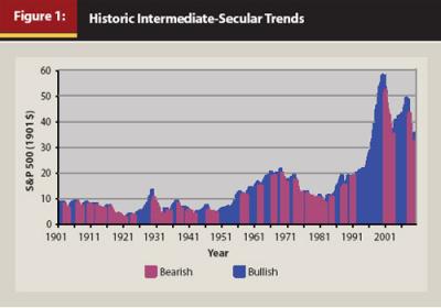
Note that the maxima and minima are of the trailing, 12-month average of the S&P 500 Index in constant dollars, whereas Figure 1 plots the actual month-to-month, constant-dollar price of the index. The graph shows that the movement of the index into a new trend can lead the average by one or two months. The current (as of December 2010) intermediate-secular bullish trend began in August of 2009.
Intermediate-Secular-Trend Distributions of the S&P 500 Index
As shown in Figure 2 and Table 1, the statistical distributions7 of monthly price-percentage change characterizing bullish and bearish periods of the S&P 500 Index are decidedly different from each other. Because human judgment was not involved in selecting the trend transition points once the criteria were set, the difference in distributions implies that market behavior trends are real, not the result of purely random variations.8 The nature of market randomness will be discussed further in a later section.
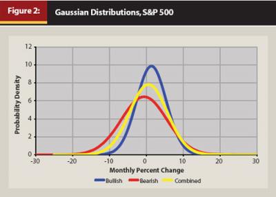
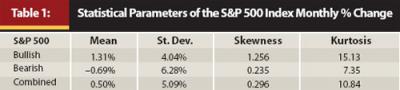
Historical data on the S&P 500 Index are readily available on the Internet from multiple sources, downloadable to a spreadsheet. One can then separate the data into bullish segments and bearish segments based on the criteria stated above. Using the mathematical power of the spreadsheet, one can determine the means, standard deviations, and other distribution descriptors of the bullish-periods data, and separately of the bearish-periods data. These are presented in Table 1 together with the combined index data (which disregard trends).9
We observe that the mean monthly percent change of the bearish distribution is 2 percentage points less than that of the bullish distribution. Also, the standard deviation of the bearish distribution is 50 percent greater than that of the bullish distribution. In bearish periods, the S&P 500 Index decreases on average month-to-month, while its volatility (a measure of risk) as reflected in its standard deviation is substantially greater than that for bullish periods.10
Actual Versus Gaussian Index Distributions
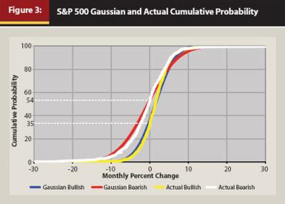
Another pertinent point is that the monthly percentage-price change statistical distributions (bullish, bearish, and combined periods) of the S&P 500 Index are not actually Gaussian. Although they appear not far from Gaussian, the differences are not trivial. Figure 3 presents the actual and Gaussian cumulative probability distributions, while Figure 4 illustrates the differences in cumulative probability percentile between the actual and Gaussian distributions.

These differences are presented here to illustrate that generally, the statistical distributions of returns of indexes and securities are not Gaussian as is assumed in many statistical models. This was pointed out years ago by Mandelbrot,11 among others. As such, in the present analysis and in the analyses of the Monte Carlo model we have been developing in-house over the past several years, only the actual distributions of the indexes are used. This is easier to do than one might expect. In the model, 22 indexes and economic indicators are tracked and analyzed. For each of these, the cumulative distributions are derived both for bullish and bearish periods using a spreadsheet as follows:
- Separate the total-return data of the index into bullish and bearish periods, one column for bullish, and one column for bearish
- Perform the operation “sort ascending” on each column
- In the column adjacent to each sorted column, number the entries sequentially and then convert this to percentiles (0th percentile –> 100th percentile) by dividing by the number of entries in the column and multiplying by 100
- Create a chart of each trend with the sorted column as the abscissa and the percentile column as the ordinate
The results will be cumulative-probability graphs of the index (or security) for bullish and bearish periods.12 This procedure can be a useful way of evaluating the behaviors of individual securities and indexes under bullish and bearish conditions.
Among these indexes, the probabilities of negative returns are greater (by 16 percent to 20 percent) under bearish conditions than under bullish. Also, whereas in the positive regions of percent change the bullish and bearish behaviors are similar, the negative regions of the bearish curves drop substantially quicker than those of the bullish curves. This implies that under bearish conditions, the primary change is in the negative direction—the cumulative-probable monthly gain does not change much, but the cumulative-probable monthly loss increases substantially.
The “80-Spread” as a Measure of Risk
Because these distributions are not Gaussian13, their standard deviations are not stable; they do not approach asymptotic values as more data are added. Standard deviations currently are used throughout the financial planning industry as a measure of volatility and risk. Because of the inherent instability of standard deviations, we have found it useful, instead, to characterize volatility and risk as the “80-spread.” We define the 80-spread as the 90th percentile value of the percent change minus the 10th percentile value of the percent change as reflected in a security’s or an index’s cumulative probability distribution. In Figures 5a and 5b the 90th percentile and 10th percentile points are plotted for some of the model’s indexes in order of increasing 80-spread value (the vertical distances between the curves).14
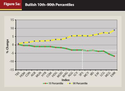
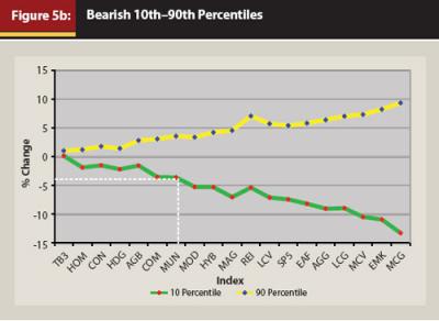
Note that, consistent with earlier observations, the 80-spread is greater under bearish conditions than under bullish, increasing even more so with the more aggressive indexes. This increase in spread is due mostly to the falling off of the 10th percentile curve. The white lines illustrate that if one wanted similar downside risk under bearish conditions as the S&P 500 Index exhibits under bullish conditions (a 10 percent probability of a 3 percent or more loss, which is equivalent to a 90 percent probability of less than a 3 percent loss in any given bullish month), one might then chose a conservative blend or municipal bonds under bearish conditions.
Is Slow-Timing the Market Practical and Effective?
The following question remains: is slow-timing the market practical and effective? Because changing allocations can involve fees and commissions, the advantages must outweigh the disadvantages. Waiting two to six months to determine that a trend change took place two to six months earlier can also be problematic, particularly because substantial market movement often takes place early in the trend. However, the greater the early movement, the less the time required to detect a trend change. To examine this question, an analysis of an actual client’s financial plan (altered to preserve confidentiality) was performed using the model, configured to represent (a) statistically bullish and bearish trend durations, (b) the times required for recognition of trend changes, (c) the bullish and bearish distributions of the model’s indexes, and (d) the different alphas and betas of the portfolio securities relative to the indexes under bullish and bearish market behaviors (the model selects the least-squares best fitting index for its alpha, beta characterization of a security).
Example: Client Analysis
Ellie Armstead, age 76, is a retired teacher and in good health. Her husband, Jon, age 75, is retired from the military and in poor health. They have an unmarried son, Jon Jr., age 44, and a married daughter, Mary, age 40, who has a daughter, Janice, age 7, and a son, Tommy, age 4. Their estate can be summarized as follows: $2,709,083 in securities, $600,000 in property, and $147,000 in debts, giving them a net worth of $3,162,083 and a total basis of $2,103,422. For the next two years their non-investment yearly income is anticipated to be $138,000, and with $172,528 yearly debt, their net yearly cash flow before taxes (not including investment income) is anticipated to be –$34,528.
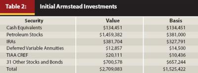
In 2012, they intend to sell their house, pay off the mortgage, and buy another house (present value of $350,00015). They also intend to buy a new car ($40,000). Their estimated yearly pre-tax cash flow during those years is –$16,000. Starting in 2020 and 2023, they intend to pay $20,000 for four years toward each of Janice’s and Tommy’s college. The money will be put into a 529 plan. Ellie’s initial security investments are presented in Table 2. They are fairly aggressive with a heavy weighting on petroleum securities having low bases.
Monte Carlo Analysis Results for Ellie’s Initial Portfolio
These data in detail were entered into the model as “Financial Strategy A” (referred to as “A” in the charts). A time horizon of 96 months was chosen, and 250 Monte Carlo runs were performed such that for each run bullish and bearish periods were statistically projected forward to the time horizon. Then Monte Carlo random draws were done on each index distribution appropriate for that bullish or bearish period, as well as for the CPI (from which inflation is computed), for the home price index and for the prime interest rate (used in conjunction with variable-rate mortgages). For these runs, no portfolio allocation changes were made with changing market trends. The results for the 8-year projection are displayed in Figure 6, with the cumulative frequency distribution of the resultant estate value shown by the red curve labeled “A$” according to the left axis, and of the mean of the yearly percent growth rate over the eight years shown by the yellow curve labeled “A%” according to the right axis.

The model analyses include determining expenses such as income and capital gains taxes, security transaction fees, and commissions in addition to the client’s claimed expenses. The estate value is net of all cash flows, having met all the client’s goals and requirements.
Note that the slopes of the curves increase sharply between the 70th percentile and the 75th percentile. This is a direct result of the market transitioning back and forth between bullish and bearish distributions. Adding more runs to the analysis does not erase or smooth out this effect. It appears to be a real consequence of market behavior. In the region below the 70th percentile the curve is governed mostly by bearish distributions, whereas above the 75th percentile it is governed mostly by bullish distributions.
This particular allocation does well at greater cumulative probabilities but has a 10 percent probability of having lost money at the end of 96 months. Each point on the curve incorporates a different, statistically selected possible future market environment and an associated projection of investment behavior. All such projections made by the model are then sorted-ascending on estate value. This results in a curve in which at lower percentiles the majority of months are projected to be bearish, whereas at higher percentiles they are projected to be bullish. We will show an example of this later.
Slow-Timing Strategy for the Armsteads
To test the market slow-timing approach with the goal of improving Ellie’s financial position, various allocation changes were proposed and tested using the model. For both bullish and bearish markets, the cash position was reduced to $110,000 (to be maintained to cover expenses), the petroleum investments were reduced by about 50 percent, the TIAA CREF investments were retained unchanged, and some variable annuity funds were switched (but not changed with changing market trends). Concerning the remaining securities: for bullish markets moderately aggressive blends were used, while for bearish markets moderately conservative blends were used. Note that the approach remains moderate partly to counter the recognition delay that exists before allocation changes can be made.16
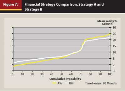
These runs are referred to as “Strategy B.” Comparative results are shown in Figure 7, which displays the mean yearly growth rates for Strategy B (white) versus Strategy A (yellow). Note that one result of slow-timing the market is that the likelihood of losing money after 96 months has disappeared—no single run had losses. Other run-series indicate that had the allocations remained bullish throughout, there would still be a 3 percent likelihood of going negative after 96 months, whereas had they remained bearish, the mean yearly growth above the 75th percentile would have been, on average, some 4 percentage points less. Strategy A is more aggressive than Strategy B as shown in the greater cumulative-probability region (Strategy B was deliberately made less aggressive than Strategy A in this region to hedge against the recognition-delay risk). However, Strategy B outperforms Strategy A under more bearish conditions without sacrificing much under more bullish conditions.
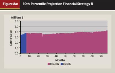
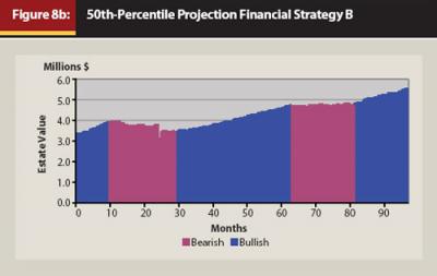
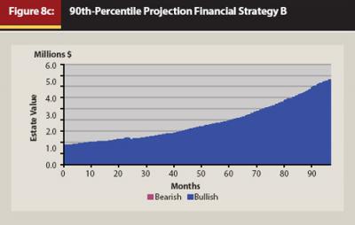
Figures 8a through 8c display the monthly projection profiles for the 10th percentile, 50th percentile, and 90th percentile runs of this projection set for Strategy B. The 10th percentile chart illustrates how the portfolio is holding its own and slightly increasing under sustained bearish conditions. The 50th percentile chart also demonstrates the effectiveness of the moderately conservative allocation under bearish conditions as well as the effectiveness of the moderately aggressive allocation under bullish conditions. The 90th percentile chart illustrates the power of this approach when the conditions are primarily bullish.
In summary, we have demonstrated that readily available data and an analytical spreadsheet can allow one to determine historical bullish and bearish trend periods based on an objective algorithm. The approach allows one, on a month-to-month basis, to ascertain trends with a lag time of two to six months. The durations of these trend periods are generally long enough for practical allocation modifications that can take advantage of the trends, and short enough for impact realization over typical financial planning horizons. Thus, slow-timing the market appears to be a reasonably advantageous approach over the “patient-hold” approach. Slow-timing allows for more effective weathering of intermediate secular bear markets and for more aggressively profiting during intermediate secular bull markets.
Final Comments
A few final comments are in order to place the findings presented here in a broader context. Whereas every effort has been made to structure the model to simulate reality as closely as is feasible, as with all such models it ultimately is an abstraction of reality based on historical patterns. Choices that had to be made in formulating the model have effects that could and do bias the model outcomes. Also, Monte Carlo statistical models generally assume statistical independence from one random draw to the next. Autocorrelation analyses of almost any publicly traded security or index will demonstrate the error of this assumption. By separating the time series into bullish and bearish behaviors, a large part of this serial dependency is accounted for.17
Monte Carlo models are intended as decision-assistance tools rather than decision-making tools. Their purpose is to inform the financial planner’s intuition and judgment. The projections made by the model represent possible future market behaviors fundamentally inherent in the market’s actual past history. Market-forcing factors that have not existed in the past century or so can and likely will arise in the future that would alter these distributions. However, in that all market investment decisions are based to some extent on the decision-maker’s sense of history and no other means is available for anticipating future forcing factors, Monte Carlo analyses based on historical data are likely to be among the better decision-assistance approaches.18 The challenge has been to represent historical patterns in a useful and effective way. We maintain that the approach presented here provides such a method, improving on previous approaches in important respects.
The algorithm used for identifying appropriate bullish and bearish periods is not sacrosanct. Variations in the threshold criteria will lead to variations in the durations of what will be labeled as a bullish or a bearish trend. These variations could lead to slight differences in the distributions of indexes, but the main fact of the validity and veracity of objectively generated bullish and bearish trends of this nature appears not to be in doubt.
Clearly, intermediate bullish and bearish trend distributions are readily applicable to efficient frontier19, 20 analyses for optimizing allocations. However, the variances and covariance matrices among the participating indexes will be different depending on whether the period is bullish or bearish. This is not typically taken into account in efficient frontier analyses. Nevertheless, many of the popular indexes have bullish and bearish distributions that are generally close enough to Gaussian that Gaussian distribution approximations should give useful efficient frontier allocations.
Much is being said these days about behavioral finance.21 Often irrational investment behavior appears to be induced by frustration—the frustration of watching your investments evaporate and feeling helpless to do anything about it. Slow-timing the market can be an effective means of reducing such frustration-induced counterproductive behaviors. However, for it to be effective, the discipline of sticking with the plan will still be necessary.
An interesting question is what the impact on the market as a whole would be if market slow-timing were to become popularly used by a great number of financial planners for their clients. Although we have not done analyses to answer this, we suspect that it would tend to decrease the volatility of bearish markets and increase the volatility of bullish markets, because a preponderance of bearish trends of more conservative investments in the market would cause it to be less volatile, while the converse would be true for bullish trends.
For financial planning clients to be able to comprehend and accept market slow-timing concepts, they will need some degree of financial literacy.22 The challenge facing the financial planner who may want to adopt the market slow-timing approach with his or her clients will be more one of client education than of available technology. As we have demonstrated, the technology is currently at hand.
Endnotes
1. Malkiel, B. G. 1996. Random Walk Down the Street. 6th ed. New York: W. W. Norton.
2. Easterling, Ed. 2005. Unexpected Returns: Understanding Secular Stock Market Cycles. 1st ed. Ft. Bragg: Cypress House.
3. Philips, Christopher B. 2008. “The Active-Passive Debate: Bear Market Performance.” Vanguard Investment Counseling Research: 3.
4. In other contexts such as day trading and fund management, market timing takes account of primary and secondary market trends.
5. An earlier version of the analytical model used here (as later described) incorporated the five phases of the business cycle based on work by Carter and Nawrocki (QInsight Group, www.qinsight.com); however, the business cycle’s primary utility is in selecting industry-sector investments. The securities market generally leads the business cycle by three to six months. Although bullish and bearish-trend security investments as described herein will initially be out of phase with the business cycle, they will be more in phase with actual market behavior.
6. The term “slow-timing” was chosen to distinguish it from other terminology applied mostly to primary-trend rotations of holdings by fund managers, and also to distinguish it from “timing the market”—attempting to forecast future market behavior.
7. The probability density (Figure 2 ordinate) is the probability percentage per unit monthly percent change of price.
8. With reference to endnote 5, the determination of business-cycle phase transitions, in addition to changes in specific economic indicators, also involves some degree of human judgment, making it less suitable for Monte Carlo types of modeling.
9. Skewness is a measure of the degree of asymmetry around the mean. Kurtosis is a measure of the peakedness of the distribution. The kurtosis of a statistical distribution is the fourth moment of the distribution.
10. During bullish periods the probability of a drop in the index in any given month is 35 percent, whereas it is 54 percent during bearish periods, as shown in Figure 3.
11. Mandelbrot, Benoit B. 1997. Fractals and Scaling in Finance. New York: Springer-Verlag. Mandelbrot categorizes states of randomness as mild (Gaussian) and wild (non-Gaussian) with some states in between. For mild randomness variances asymptotically approach real values; for wild randomness they approach infinity. He points out that stock variations are characterized best by the wild-randomness state.
12. The model additionally determines the principal effects of correlations among the indexes. This affords a deeper and more complex analysis than that described above. Also, each resultant distribution is fitted analytically by two 6th-order polynomials plus terminal-region linear fittings.
13. See endnote 11.
14. In Figures 5a and 5b the following abbreviations are employed: S&P (SP5), Russell (LCV, LCG, MCV, MCG), BarCap (AGB, HYB, MUN), MSCI (EAF, EMK), Dow Jones (REI and CON, COM, MOD, MAG & AGG blends), Credit Suisse Tremont (HDG), Citi (TB3), Bureau of Labor Statistics (CPI).
15. The model statistically projects the Standard & Poor’s home price index and the consumer price index from which the yearly inflation rate is computed. This information is used in the model to project monthly, then present values of the houses that Ellie intends to sell and purchase in 24 months.
16. In reality, trend changes and recognition delay times are directly the result of market behavior—the market beginning to behave according to a new trend. However, in the model, at this time, trend durations and recognition periods are statistically computed by the model based on historical trend-duration and recognition-duration frequency data.
17. Even though month-to-month index serial correlations persist for bullish and bearish trends (generally ≤ ±10 percent out to 12 months of relative displacement) they are not directly reflected in the model; however, the division of the data into separate trend distributions accounts for much of the trend bias such that the remaining statistical behavior ≥ 90 percent) is essentially random. Also, cross correlations among indexes are reflected in the model such that the statistics generated by the model are close to the original statistics, including index cross correlations.
18. It should be noted that a valid alternative analytical modeling approach is to run the model using actual long-term historical market behavioral data (as opposed to Monte Carlo, statistically generated data based on long-term historical market behavioral data). A discussion of the pros and cons of both analytical approaches is beyond the scope and emphasis of this paper.
19. Markowitz, Harry M. 1998. Portfolio Selection. Cambridge, MA: Blackwell.
20. See Richard and Robert Michaud’s papers (www.newfrontieradvisors.com) for leading efficient frontier research.
21. For example: Mitchell, Donna. 2010. “The Pioneer.” Financial Planning 40, 7.
22. Mark Cohen and Wes Burnett recently wrote a book on financial literacy intended for younger adults but applicable to all: Cohen, I. Mark and Weston D. Burnett, 2010. Lessons to My Children. Great Falls, VA: LINX.