Estimating Credit Risk and Illiquidity Risk in Guaranteed Investment Products

Journal of Financial Planning: July 2012

James X. Xiong, Ph.D., CFA, is a senior research consultant at Morningstar Investment Management in Chicago, Illinois. (james.xiong@morningstar.com)

Thomas M. Idzorek, CFA, is president of Morningstar’s global investment management division. (thomas.idzorek@morningstar.com)

Executive Summary

• Guaranteed investment products, including stable value funds, guaranteed investment contracts (GICs), synthetic GICs, bank investment contracts (BICs), deferred fixed annuities, etc., are offered in many defined contribution plans in the United States.
• These downside guaranteed products can vary significantly from product type to product type, as well as within a given product type. But many of these products share some common characteristics that are not found in traditional marked-to-market products.
• This paper establishes a flexible framework for estimating credit risk and illiquidity risk for guaranteed products, so their “true” risks are reflected in the inputs to asset-allocation-oriented optimizations.
• Ignoring or inaccurately estimating illiquidity risk and credit risk can lead to an unjustified preference for guaranteed products.

Guaranteed products include stable value funds, guaranteed investment contracts (GICs), synthetic GICs, bank investment contract (BICs), and deferred fixed annuities, to name a few. They are offered in many defined contribution plans in the United States. Many of these products appear to have low risk—as conventionally measured from traded and market-based instruments—because the credited returns are set based on rules and formulas rather than marked to market. In order to evaluate such products, to compare them to one another, and to determine an appropriate allocation to a guaranteed investment product, it is important to estimate the true risk of these products.

Despite the popularity of guaranteed products, the practitioner literature offers surprisingly little guidance in their evaluation, risk estimation, and ultimately, their role in a diversified asset allocation portfolio. Numerous academic researchers have priced-out and valued structured products on a stand-alone basis, but have been mostly silent on the optimal allocation and role in the optimal portfolio. The calculation of a risk-neutral price is simply too arduous for most practitioners.

One important exception in the void of practitioner-oriented papers is Babbel and Herce (2011), which examines the performance of stable value funds since their inception in 1973. It analyzes the performance of stable value funds using mean-variance analysis, Sharpe and Sortino ratio analyses, stochastic dominance analysis, and multi-period portfolio optimization (or intertemporal optimization). All of these historical analyses suggest that stable value funds dominate short-term government/credit bond funds and cash, and that stable value funds often occupy a significant position in optimal portfolios across a broad range of risk-aversion levels. In this case, the domination of stable value funds comes from a similar return but with a significantly lower standard deviation of returns—a standard deviation that we believe does not reflect the true risk of the investment.

Comparing the volatility of a marked-to-market asset (an asset whose price is determined by the market) to that of a rules-based product that is not marked to market is not an apples to apples comparison. Some continue to argue that the volatility of a guaranteed product that is experienced by the investors should be used for asset allocation and/or portfolio construction. We believe such a view fails to consider the true risk of the products to investors, and makes meaningful comparisons between two rules-based products challenging. For example, the coupon payments associated with Lehman Brothers-issued structured products had no standard deviation until Lehman’s bankruptcy in 2008 (see Zhang 2010).

Credit and Illiquidity Risks

For guaranteed investment products, credit risks are extremely relevant, especially in the case of a single issuer. For example, traditional GICs are typically backed by the financial health of the insurance company issuing the contract, not by the federal government. Therefore a GIC is only as good as the insurance company that issues the contract. While there have been very few meltdowns of insurance companies, the infamous failures of Executive Life and Mutual Benefit Life in 1991 forced pension fund managers and 401(k) plan investors to rethink GICs and to reevaluate the credit risk associated with them.

Another type of risk associated with guaranteed products is illiquidity risk. Some guaranteed products, but not all, have restrictions or penalties on withdrawals, which limit immediate access to the investor’s money and limit the investor’s ability to rebalance their overall portfolio toward their target asset allocation. From one perspective, this illiquidity helps make the guaranteed investment product safer because it can mitigate a “run on the bank” during extreme market events and potential arbitrage situations. To some degree, it is this illiquidity that enables the product manufacturer to guarantee the principle. From a negative perspective, because of this inability to rebalance, the actual or realized asset allocation may be significantly different from the target, and thus, the risk characteristics will be different from those of the target. In other words, the inability to rebalance introduces uncertainty around the actual asset allocation an investor might have at a given time; hence, there will be uncertainty in the risk characteristics of the portfolio.

Leland (2000) shows that there is a “cost” associated with an undesired overall risk exposure caused by the inability to rebalance that can be estimated as the present value of expected loss in utility. Systematically rebalancing a portfolio toward a target is in fact a type of investment strategy in which one systematically sells assets that have appreciated in price and buys assets that have depreciated in price. It is a contrarian investment strategy that is expected to earn a small liquidity premium because the investor is systematically supplying liquidity to the market. Empirical studies, such as Buetow et al. (2002), show that disciplined rebalancing can enhance returns and control risk. This point was also made by Milevsky (2004) and Browne, Milevsky, and Salisbury (2003), and they subsequently derived the liquidity premium required to compensate for the utility loss resulting from the inability to rebalance.

Willenbrock (2011) demonstrates that the underlying source of a “diversification return” is rebalancing. If each individual asset in a portfolio has a geometric average return of zero, the non-rebalanced or buy-and-hold portfolio will have a geometric mean return of zero. In contrast, the geometric return of a rebalanced portfolio made up of the same zero returning assets will earn a positive return. That positive incremental return is the diversification return.

A complete analysis of a guaranteed product must go beyond the artificially smoothed historical returns, incorporating credit risk and illiquidity risk into the analysis. In an optimization setting, the failure to incorporate these two additional risks will undoubtedly lead to an incomplete analysis, and most likely, allocations to guaranteed product that are too large relative to their complete risk and return characteristics. This paper explores ways to estimate credit risk and illiquidity risk for guaranteed products, so their “true” risks are reflected in the inputs to the optimizations.

Overview of Guaranteed Products

Guaranteed products are prevalent in 401(k) retirement plans. Unfortunately, the guaranteed product world is one in which the term “stable value fund” often serves as a catch-all term for a wide variety of these downside-protected products, most of which are not mutual funds at all. Throughout the rest of the paper we use “guaranteed products” to refer to these types of products with option-like asymmetric expected payouts.

An important distinction among the products is whether the invested assets are held in a segregated, separate account or in a general account. In a separate account structure the investor bears investment performance risk and purchases an insurance “wrapper” that provides the guarantee. Because the assets are held in a separate account they are not subject to potential creditor claims against the product manufacturer. For general account products, the assets are invested in the general account and the credited returns and principal are subject to the claims-paying ability of the company in question.

Here we give a brief introduction to the most common types of guaranteed products.

Stable Value Funds. Stable value funds usually offer smoothed returns that are at a level similar to those of the BarCap U.S. Aggregate Bond Index. The assets of a stable value fund are held in a separate account created by the insurance company, mutual fund company, or bank/trust company creating the fund. Stable value funds invest primarily in guaranteed investment contracts or GICs. In the stable value fund structure, the fund manager can spread default risk over multiple GIC issuers.

Guaranteed Investment Contracts (GICs). GICs, primarily offered by banks and insurance companies, are contracts in which the issuer agrees to pay a predetermined interest rate and principal. The interest payments and, more importantly, principal are subject to default risk. In theory, this is a spread product in which the issuer invests more aggressively to earn a spread over time. The return of a general-account-based GIC should be higher than either a separate-account-based GIC or a synthetic GIC (discussed below), because of the default risk associated with the principal. For details, see Kleiman and Sahu (1992).

Synthetic GICs. In this case, the investor retains ownership and control of the underlying investment (usually high-quality bonds) and purchases a “wrapper” from an insurance company. The wrapper can cover all or part of the assets. Most commonly, the wrapper guarantees that the principal will not go down and the minimum return (floor) is above 0 percent.

Bank Investment Contracts (BICs). BICs are similar to GICs, but the underlying assets are held in trust protecting them from other potential obligations of the issuer. In contrast, the assets invested in a GIC are often part of a general account and thus could be impaired by the well-being of the general account. A BIC may or may not be covered by FDIC insurance.

Deferred Fixed Annuity. A deferred fixed annuity is an insurance contract, usually between an individual investor and the insurance company. The invested money is placed in the insurance company’s general account and invested as the insurance company sees fit, and is thus subject to default risk (ignoring any government guarantees). Each contribution into the deferred fixed annuity will be credited with the current interest rate as declared by the issuer. The initial interest rate is declared in advance and guaranteed for some length of time (for example, one, three, or five years). Following the expiration of the guaranteed period, most deferred fixed annuity contracts will continue to be credited with a slightly lower-than-market interest rate, with periodic adjustments. As with all deferred annuities, the holder has the right to annuitize the contract value.

These guaranteed products can vary from product to product, but they all share some common characteristics:

• The credited returns are set by formulas, and are not marked to market
• The volatility—as measured by standard deviation—of the returns is lower than the volatility of money market funds or cash (except in extreme circumstances)
• There is a guaranteed minimum return (floor), for example, 0 percent or 2 percent¹
• Liquidity constraints can exist from 1 year to 10 years
• The credit risk of the issuer(s) cannot be ignored

To help generalize our analysis to a wide variety of the potential guaranteed products, we create a hypothetical guaranteed product (HGP) that has many of the common characteristics of the products observed in the marketplace. The historical returns are based on actual products that will remain anonymous. For our purposes, HGP is a guaranteed product that promises to preserve the principal value, to pay a minimum guaranteed interest rate of 2 percent (with the opportunity for additional amounts), and to let participants choose lifetime income payments when they retire. We should note that in today’s low interest rate environment, a 2 percent guaranteed interest rate is relatively generous, and was certainly more common in the past. Clearly not all guaranteed products share these exact characteristics. Our goal is to establish and apply a flexible framework for estimating credit risk and illiquidity risk for guaranteed products that in turn can be modified and extended to account for different product features. We encourage practitioners to move forward with the spirit of the analysis and enhance it to meet their particular needs.

Historical Analyses

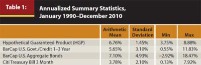
We start by identifying the arithmetic mean return, standard deviation of realized returns, and the minimum and maximum return for historical crediting rates of HGP in Table 1. Within the parlance of the guaranteed product world in which returns are determined by rules (the amount received by the investor is typically the minimum guaranteed return plus an additional amount), the term “crediting rate” is often used rather than “return” or “interest rate.” For comparison purposes, we provide the equivalent summary statistics for the same period for the BarCap U.S. Government/Credit 1–3 Year Bond Index, BarCap U.S. Aggregate Bond Index, and the Citigroup Treasury Bill 3 Month Index. From Table 1, we can see that the historical mean return for HGP from 1990 to 2010 is comparable to the BarCap U.S. Aggregate Bond Index and it outperforms a typical bond fund (with an expense of about 65 bps²) by 31 bps; however, the standard deviations of returns for HGP are about 3.5 percentage points lower than the standard deviation of the BarCap U.S. Aggregate Bond Index. The volatility of HGP is even lower than that of the cash. As a result, the Sharpe ratio of HGP is much higher than the aggregate bond index based on empirical data.

As one would expect given its apparent superior Sharpe ratio,³ HGP tends to dominate the safe or fixed-income allocations of the efficient frontier. Again, as we pointed out earlier, the artificially low standard deviations of the historically credited returns belies the true risk of HGP. To perform a meaningful mean-variance analysis, we need to adjust the standard deviation number to account for both credit risk and illiquidity risk.

Forward-Looking Analyses

When attempting to determine an appropriate asset allocation for the future, we prefer to use forward-looking capital market assumptions.

While the pertinence to the end investor of how the actual assets of a guaranteed product are invested depends on the product structure, the composition of the underlying investments that we assumed for HGP are 90 percent general fixed income (BarCap U.S. Aggregate Bond TR), 4 percent domestic equities (S&P 500 TR), 4 percent institutional real estate (NAREIT-Equity TR), and 2 percent cash (CG U.S. Domestic 3 Mo T-bill).⁴ Experience tells us that this is not that different from how the assets of a deferred fixed annuity might be invested within an insurance company’s general account. Certainly not all general accounts are invested the same, and for our purpose we want to back out the equity-centric asset allocations associated with life insurance investments and focus on the portion of the general account funding the guaranteed product. Historically, the mini-portfolio of sorts in HGP has produced a superior return at a slightly lower risk level than a portfolio consisting of 100 percent BarCap U.S. Aggregate Bond Index. Again, you can see that the issuer of such a product hopes to earn a spread over time—time is the issuer’s friend.

Table 2 shows an example of Ibbotson forward-looking capital market assumptions for five assets: large cap, mid-small cap, international equity, bonds, and HGP. At this stage in our analysis, the mean and standard deviation of HGP are calculated based on the underlying asset allocation of HGP, as detailed above.

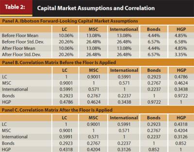
The top part of Panel A of Table 2 shows the unconditional mean and standard deviation, while the bottom part of Panel A shows the modified mean and standard deviation after adjusting for the 2.0 percent guaranteed minimum return floor.⁵ The floor return can be a valuable hedge against downside risk. The tradeoff is that the upside gain is typically capped. This is similar to a collar strategy that sells a call option and buys a put option.

As a result of applying the floor, the standard deviation of HGP is significantly reduced from 6.58 percent to 3.35 percent, an amount that still exceeds the historical standard deviation of most of these types of guaranteed products. Panels B and C of Table 2 show the correlation matrix before and after the floor was applied to the HGP.

It is important to note that our analyses are performed at the asset-class level, not at the fund or product level. The expenses and management fees must be considered at the fund or product level.

As shown in Panels B and C, the correlation between HGP and bonds is 12 percentage points lower after the floor is applied, while the correlations between HGP and equity asset classes are about 3–4 percentage points lower after the floor is applied. While the proper application of the floor is a necessary first step to eventually arriving at an appropriate standard deviation of returns estimate for HGP, we have yet to account for credit and illiquidity risk.

Estimating Credit Risk

For our purposes, credit risk refers to the default risk of the issuer of the guaranteed investment product. Assuming equal credit worthiness, catastrophic credit risk diminishes substantially when it is spread across multiple issuers, such as a true stable value mutual fund that owns multiple GICs from multiple issuers, but it is extremely important for any investments with single-carrier credit risk, such as a deferred fixed annuity or other general account backed product. Examining a debtor’s ability to repay its financial obligations is critical to the valuation and asset allocation of debt portfolios.

For more than a century, the big three bond-rating agencies—Moody’s, Standard & Poor’s, and Fitch—have been the unchallenged arbiters of corporate creditworthiness. Rating references are embedded in hundreds of guidelines, laws, and private contracts that affect a broad range of financial concerns. The financial crisis in 2008, however, revealed a weakness in the credit-rating agencies’ models: their ratings are backward-looking because they are predicated on historical data that is observed at a discrete point in time. Given this constraint, the agencies have not been able to react quickly to rapid changes in a creditor’s financial health. Hence, evidence of accounting fraud in a company’s financial statements may elude their scrutiny. Also, the agencies have demonstrated that they remain ill-equipped to assess the risks of some complex, structured products. The 2008 crisis also revealed the importance of hedging the complex risks taken on by insurance companies—a few thrived while others bumped up against capital requirements. To our knowledge, the rating agencies struggle to understand the complicated risks created by the various insurance products as well as the quality of the various hedging programs that can substantially mitigate such risks.

There are various ways to estimate the credit risk of a guaranteed investment product. In this paper, we choose to use Morningstar’s distance to default (DTD) to model the issuer’s credit risk (see the appendix for more details). Our goal is to adjust the guaranteed product’s risk for the credit risk by using the DTD measure.

Next, we need to know more about the guaranteed product. In particular, we need to estimate the expected loss to investors should the issuer default. This can be a difficult task, but detailed analysis on the issuer’s financial status can offer a reasonable estimate. For general account products, the default loss is unlikely to be 100 percent because holders of guaranteed investment products usually come before the equity holders. If no data is available, we assume that the default loss is 30 percent for the guaranteed investment product.⁶ As we will show later, one can perform scenario analyses by assuming different default losses, for example, 25 percent. This loss will be used to adjust the guaranteed product’s risk for the credit risk. As in our simplified example given in the appendix, where the DTD for the issuer is 2.5, let’s assume an investor had purchased a guaranteed product with a value of $10. Coupling this with our assumed expected loss in a default of 30 percent, along with the probability of a default of 0.62 percent, the expected loss for the investor is about 2 cents.

Now the question becomes how to find a standard deviation of returns estimate for the guaranteed product so that it has a 0.62 percent chance to lose 30 percent. By doing this, we are able to incorporate the credit risk of HGP into a corresponding standard deviation of returns estimate that is arguably more appropriate for use in a mean-variance optimizer. This estimate can be made as long as a return distribution is assumed and the other three moments of the return distribution are known or assumed. We do this by treating the guaranteed product as a type of fixed-income investment. The distribution of the fixed income is assumed to follow a skewed and fat-tailed model—truncated Lévy flight model (Xiong 2010). We run Monte Carlo simulations (in which returns follow a truncated Lévy flight distribution rather than a normal distribution) to establish the relationship between the probability of a 30 percent loss in one year and the standard deviation of returns estimate by fixing the other three moments: mean, skewness, and kurtosis. The last two columns of Table 3 show the estimated standard deviations of returns for the 30 percent and 25 percent expected default losses that correspond to the different distance-to-default/probability-of-default levels, respectively.

From Table 3, we see that in our example the DTD of 3.25 corresponds to an estimated standard deviation of returns of 6.65 percent (5.70 percent) for a 30 percent (25 percent) default loss. When the DTD is less than 2.5, the probability of default is too great to ignore. If the DTD is greater than 6, the default is remote. Because the DTD changes with the stock price of the issuer, we can monitor and dynamically adjust for the credit risk as necessary.

As we mentioned earlier, the default loss is an important parameter to estimate. If the default loss is less (more) than 30 percent, the risk level in Table 3 will be correspondingly lower (higher). A lower (higher) default loss indicates that a lower (higher) adjustment for the credit risk is needed. The last column in Table 3 shows that if the expected default loss is 25 percent rather than 30 percent, the risk level or standard deviation is about 1–2 percentage points lower.

While the DTD method is our preferred method for estimating a standard deviation of returns that accounts for credit risk because it is a forward-looking estimate, it cannot be calculated for non-publicly traded companies. If the DTD value or similar estimate is not available, we use the average of the credit ratings from the three agencies (Moody’s, Standard & Poor’s, and Fitch) for the issuer in question, and use the credit migration matrix from Schuermann (2008) to estimate the probability to default (see Table 4).

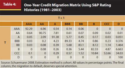
Table 4 shows that a current credit rating of AAA has a 92.29 percent chance to stay in AAA and a 0 percent probability of default in the next year. However, this should be viewed cautiously. For example, AIG had a credit rating of AAA until September 19, 2008. Had it not been for the U.S. government bailout, AIG would have been forced to file for bankruptcy protection. In practice, we use professional judgment to modify the various probabilities, such as assigning a small but non-zero probability (0.001 percent) of default to AAA.

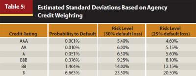
In Table 5, for each of the probabilities of default associated with the ratings coupled with our base case 30 percent expected loss during a default, we rerun our Monte Carlo simulation to estimate the standard deviation of returns for the guaranteed product. Notice that a guaranteed product with single-carrier credit risk from a AA-rated private insurer has a 0.01 percent probability of default, which corresponds to an estimated standard deviation of returns of 6.0 percent. In the final column of Table 5, we once again show the estimated standard deviations based on expected loss of 25 percent during a default. We believe a strong argument can be made that these modified estimates of standard deviation that incorporate creditor risk are significantly more appropriate estimates in a forward-looking context. In almost all cases the estimated standard deviations of returns are significantly higher than the realized standard deviations of the past.

Estimating Illiquidity Risk

Next, we turn to illiquidity risk. While clearly illiquidity risk involves the haircut one must receive for demanding immediate liquidity (should liquidity even be available), our adjustment for illiquidity risk focuses on the utility loss that results from the inability to rebalance the portfolio across time. In the presence of rebalancing restrictions—the type of restrictions embedded in many guaranteed income products—assets with relatively poor past returns will see their weights fall, while the ones with relatively high returns will increase in weight. The implication is that both portfolio composition and portfolio total risk will change across time and will not necessarily equal those of the desired target asset allocation.

To illustrate, consider the impact of the 2008 financial crisis. During the crisis, fixed-income asset classes dramatically outperformed equity asset classes. If one was unable to rebalance, the realized or actual asset allocation drifted away from the target, overweighting fixed-income asset classes and underweighting equity asset classes. As a result, the total risk level of the portfolio would be much lower than the target risk at the end of the crisis. In this example, as the market fell, the inability to rebalance helped investors, but it hurt them during the rebound.

Withdrawals make the problem even worse because the withdrawals must come from liquid assets; thus, the portfolio will deviate from the target asset allocation further. Lu and Mitchell (2010) examine the withdrawal behavior in 401(k) plans. They find that most withdrawals are less than 20 percent of the maximum allowable withdrawal. Additionally, they find that participants are most likely to take loans between ages 35 and 45.

We estimate the illiquidity risk by computing what economists refer to as “utility loss,” which in this case is the decrease in utility caused by the inability to fully rebalance the portfolio. For most of us, we should think of “utility” as a complex definition of “good” that takes into consideration the trade-off between features we like (for example, the ability to consume) and features we don’t like (for example, the risk of not being able to consume), and weights the features accordingly. Browne, Milevsky, and Salisbury (2003) provide a theoretical framework to calculate the liquidity premium demanded by the holders of illiquid assets to compensate for the utility welfare loss. Instead of adjusting the expected return as done in Browne, Milevsky, and Salisbury (2003), we adjust the standard deviation of the illiquid asset so that the utility of the non-rebalanced portfolio (the static portfolio with the standard deviation not adjusted for the illiquid asset) equals that of the rebalanced portfolio (the dynamic portfolio with the standard deviation adjusted up for the illiquid asset).

We provide the following equations:

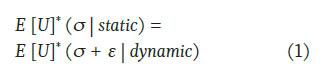
In Equation 1, E [U]* indicates the maximal expected utility. s is the standard deviation of the illiquid asset, and here we assume it equals 3.35 percent as shown in Table 2 (after the floor is applied). e is the illiquidity risk adjustment that needs to be estimated. ε is the amount to which the standard deviation needs to be adjusted in order to satisfy Equation 1. The illiquidity-adjusted total risk is the combination of the two (δ + ε).

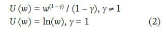
We assume the utility for an investor with constant relative risk aversion preferences for uncertain wealth for a given horizon is modeled by Equation 2.

To simplify the solving process in Equation 1, we assume that there are only two assets, the large-cap stocks (LC) shown in Table 2 and HGP. LC is the liquid asset, and HGP is the illiquid asset. γ is selected as 2.8 based on Browne, Milevsky, and Salisbury (2003) to maximize the illiquidity risk adjustment because we want to make our adjustments conservative.

We employ Monte Carlo simulations to solve the illiquidity risk (ε) because of the complexity of Equation 1. The utility of cumulative wealth is calculated at the end of the liquidity-constrained horizon (for example, seven years) for each simulated return path. In total, we simulated 2,000 return paths. The averaged utility is then maximized for both static and dynamic portfolios to derive the illiquidity risk adjustment (e).

The simulated results are shown in Table 6, in which we calculate the illiquidity risk adjustment for different liquidity constraints (5 years, 7 years, or 10 years) and different withdrawal scenarios (no withdrawals, 10 percent, 20 percent, 30 percent, and 40 percent). The withdrawals are assumed to be taken in the first four years to simulate a case of supporting a college student for four years. To make the withdrawals comparable for the two portfolios (static and dynamic), we assume that the annual withdrawals are the same in dollar amounts for four years. For example, given the initial wealth of $100, each year’s withdrawal is $10 ($40 for the four years) for the 40 percent withdrawal scenario.

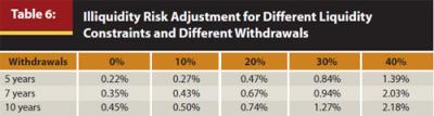
Table 6 shows that the illiquidity risk adjustment is about 0.35 percent without withdrawals for a seven-year, liquidity-constrained horizon. However, it is increased to 2.03 percent when withdrawals of 40 percent are taken. The illiquidity-adjusted total risk is therefore 3.7 percent (0.35 percent + 3.35 percent) for the 0 percent withdrawal case and 5.38 percent (2.03 percent + 3.35 percent) for the 40 percent withdrawal case. In general, a longer liquidity-constrained horizon or a larger withdrawal will increase the illiquidity risk because rebalancing is restricted to a larger degree. Conversely, a shorter liquidity-constrained horizon or a smaller withdrawal will decrease the illiquidity risk.

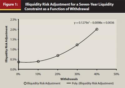
Figure 1 plots the illiquidity risk adjustment for the seven-year, liquidity-constrained horizon against different withdrawal scenarios shown in Table 6. Once again, the illiquidity risk adjustment (ε) is the amount to which the standard deviation needs to be adjusted in order to satisfy Equation 1. It is interesting to note the curve can be fit by a polynomial function with an order of 2 very well.

Putting the Pieces Together

In this paper, we have developed two very different methods for estimating the standard deviation of returns of HPG: one based on credit risk and one based on illiquidity risk. For credit risk, we developed a method based on Morningstar’s distance-to-default measure, or for cases in which the distance to default is unavailable, agencies’ credit ratings, to infer the credit risk-adjusted standard deviation of HGP. For illiquidity risk, we used Monte Carlo simulation to quantify the amount of illiquidity risk adjustment by computing the utility loss resulting from the inability to rebalance. In this section we bring these two separate pieces together in a process designed to determine an appropriate allocation to HGP.

The steps are as follows:

1. Estimate the credit risk-adjusted standard deviation of returns of HGP
2. Estimate the illiquidity risk-adjusted standard deviation of return of HGP
3. Select the larger estimate of risk-adjusted standard deviation from Steps 1 and 2 for HGP
4. Using Step 3’s standard deviation estimate for HGP, perform your preferred asset allocation optimization, such as resampled mean-variance or mean-CVaR optimization

To demonstrate Step 3 in which we select the higher standard deviation from Steps 1 and 2, we assume HGP comes from a private company with a credit rating of AAA. As shown in Table 5, the estimated credit risk-adjusted standard deviation is 5.4 percent for a default loss of 30 percent, and 4.6 percent for a default loss of 25 percent. As shown in Table 6, the estimated illiquidity-adjusted risk is 3.7 percent (no withdrawal) and 5.38 percent (40 percent withdrawal) for a seven-year liquidity constraint. Which number to choose depends on the estimates on default loss, liquidity-constrained horizon, and withdrawals.

If the default loss is 30 percent, liquidity-constrained horizon is seven years, and there is no withdrawal, our final risk-adjusted standard deviation for HGP is 5.4 percent (max(5.4 percent, 3.7 percent)). If the default loss is 25 percent, liquidity-constrained horizon is seven years, and the withdrawal is 40 percent, our final risk-adjusted standard deviation for HGP is 5.38 percent (=max(4.6 percent, 5.38 percent)).

By choosing the more cautious estimate of true risk, we are focusing on the weakest link in the chain. If the credit rating of the issuer for HGP is significantly downgraded, the credit risk-adjusted estimate will most likely exceed the illiquidity risk-adjusted estimate, and thus a lower allocation to HGP is warranted.

It can be seen that the optimal allocation to HGP is sensitive to a number of variables. Our framework provides a starting point to quantitatively assess the true risk of guaranteed investment products. In practice, it should be combined with other quantitative or qualitative judgments to make the process more robust.

Conclusions

Guaranteed investment products are fundamentally different from typical marked-to-market investments, and as such, new techniques are required. Guaranteed investment products contain two unique hidden risks—credit risk and illiquidity risk—that are not necessarily reflected in the standard deviation of historical returns. We have developed two very different approaches to estimating what we believe to be more accurate standard deviation estimates that incorporate credit risk and illiquidity risk.

The credit risk-adjusted standard deviation is based on a market-based, distance-to-default estimate or by extrapolating from the credit ratings issued by the various rating agencies, both of which lead to an estimate of the probability of default. Based on the assumed haircut one would experience during a default coupled with the probability of default in a given horizon, we infer the credit risk-adjusted estimate of standard deviation.

The illiquidity risk-adjusted standard deviation is based on the idea that liquidity constraints can result in a utility welfare loss due to the inability to rebalance. The illiquidity risk to be adjusted depends on the liquidity-constrained horizon and withdrawals during that horizon.

We believe both of these adjusted estimates of standard deviation do a better job of reflecting the true risk of these guaranteed investment products into a single statistic that most practitioners are comfortable using. Additionally, these adjustments help put guaranteed investment products on an even playing field with marked-to-market assets and asset classes as it pertains to a single measure of risk, enabling more appropriate comparisons. Finally, we believe these adjusted standard deviation estimates can serve as better inputs into an asset allocation optimization, resulting in asset allocations that don’t unduly favor guaranteed investment products.

Endnotes

1. In the current low interest environment, typical minimum guaranteed returns on new products are 0 percent. One exception is within the 403(b) space where, due to various rules, the required floor must exceed 0 percent.
2. At the time of this writing, the management fee of the PIMCO Investment Grade Corp Bond A fund was 0.65 percent.
3. The Sharpe ratio may not be an appropriate measure given that the return distribution of HGP is likely not normally distributed.
4. The National Association of Insurance Commissioners and the Center for Insurance Policy and Research publish more detailed asset allocations for the industry. A recent example is available from www.naic.org/capital_ markets_archive/110819.htm.
5. More specifically, a Monte Carlo simulation, in which the underlying asset classes of HGP were assumed to follow a multivariate truncated Lévy flight distribution (see Xiong 2010 for details), was used to generate a return series with the appropriate starting summary statistics, and then returns below 2.0 percent were automatically set to 2.0 percent. The returns are also capped so that the expected return remains 4.85 percent. Lastly, the modified summary statistics were calculated.
6. In most cases, additional information will be available enabling the practitioner to fine tune the expected loss should a default occur, which might include account type (general account versus separate account), various reserves, an assessment of hedging programs, etc. Our 30 percent estimate is based on GAO-11-400, “Retirement Income: Ensuring Income Throughout Retirement Requires Difficult Choices,” from June 7, 2011. Footnote 67 in this report states, “Although experts said that Executive Life Insurance Company had high ratings from certain rating agencies—A.M. Best, Moody’s, and Standard & Poor’s—prior to its insolvency, we reported that 44,000 retirees with Executive Life had received only 70 percent of their promised monthly annuity payments for almost 13 months after California regulators seized control of the company.”

References

Babbel, David F., and Miguel A. Herce. 2011. “Stable Value Funds: Performance to Date.” Unpublished paper.

Black, F., and M. Scholes. 1973. “The Pricing of Options and Corporate Liabilities.” Journal of Political Economy 81: 637–654.

Browne, S., M. A. Milevsky, and T. S. Salisbury. 2003. “Asset Allocation and the Liquidity Premium for Illiquid Annuities.” Journal of Risk and Insurance 70, 3: 509–526.

Buetow, Gerald W. Jr., Ronald Sellers, Donald Trotter, Elaine Hunt, and Willie A. Whipple Jr. 2002. “The Benefits of Rebalancing.” Journal of Portfolio Management 28, 2 (Winter): 23–32.

Kleiman, Robert T., and Anandi P. Sahu. 1992. “The ABCs of GICs for Retirement Investing.” AAII Journal (March).

Leland, Hayne E. 2000. “Optimal Portfolio Implementation with Transaction Costs and Capital Gains Taxes.” University of California at Berkeley, Haas School of Business, Working Paper.

Lu, Timothy Jun, and Olivia S. Mitchell. 2010. “Borrowing from Yourself: The Determinants of 401(k) Loan Patterns.” Unpublished paper.

Merton, R. 1973. “Rational Theory of Option Pricing.” Bell Journal of Economics and Management Science 4: 141–183.

Milevsky, Moshe Arye. 2004. “Illiquid Asset Allocation and Policy Weights: How Far Can They Deviate?” Journal of Wealth Management 7, 3: 27–34.

Miller, Warren. 2009. “Comparing Models of Corporate Bankruptcy Prediction: Distance to Default vs. Z-Score.” Morningstar Methodology Paper.

Schuermann, Til. 2008. “Credit Migration Matrix.” In Encyclopedia of Quantitative Risk Analysis and Assessment, Edward L. Melnick and Brian S. Everitt, eds. Hoboken, NJ: John Wiley & Sons.

Willenbrock, Scott. 2011. “Diversification Return, Portfolio Rebalancing, and the Commodity Return Puzzle.” Financial Analysts Journal 67, 4: 42–49.

Xiong, James X. 2010. “Using Truncated Lévy Flight to Estimate Downside Risk.” Journal of Risk Management in Financial Institutions 3, 3: 231–242.

Xiong, James X., and Thomas Idzorek. 2011. “The Impact of Skewness and Fat Tails on the Asset Allocation Decision.” Financial Analysts Journal. 67, 2: 23–35.

Zhang, Miao. 2010. “Hong Kong Investors’ Experience with Structured Financial Products: Financial Literacy, Learning, and Social Networks.” Student dissertation, The Graduate School of the University of Hong Kong.