Journal of Financial Planning: February 2011
David M. Blanchett, CFP®, CLU, AIFA®, QPA, CFA, is the director of consulting and investment research for the Retirement Plan Consulting Group at Unified Trust Company in Lexington, Kentucky.
Executive Summary
- There are important “costs” an adviser should consider when implementing a tactical asset allocation strategy for a client.
- The research conducted for this paper suggests that in order to achieve similar risk-adjusted performance as a static portfolio with the same equity allocation, one must be able to correctly select the outperforming asset class (either bond or equity) approximately 66 percent of the time, ignoring taxes.
- In order to achieve similar risk-adjusted performance as a static portfolio with the same equity allocation on an after-tax basis, one must be able to correctly select the outperforming asset class approximately 70 percent of the time.
- The likelihood of a tactical approach outperforming a static allocation decreases further when considering additional costs incurred by tactical investors, such as additional trading expenses.
- Therefore, a long-term static allocation strategy is likely the approach that will lead to higher risk-adjusted performance for the majority of investors.
When it is not in our power to determine what is true, we ought to follow what is most probable.
~ Rene Descartes
These are tough times for buy-and-hold investing. With equity markets down 35 percent in 2008 and up 25 percent in 2009, many advisers have started looking for “better” ways to invest in order to overcome the “shortcomings” of buy-and-hold investing. The alternative to buy-and-hold investing, or a static asset allocation policy, is a tactical approach, where changes are made to the allocation in response to market forecasts. While there are a variety of types, methods, and approaches to tactical investing, little research has been devoted to exploring the potential costs of implementing a tactical strategy from a portfolio efficiency and return perspective. This paper will explore two quantitative costs: increased portfolio risk and the impact of the additional trading on after-tax returns, and briefly discuss three qualitative risks: the cost of benchmark variation, the difficulty of identifying luck and skill, and additional trading expenses. The purpose is to provide the reader with guidance as to what level of certainty (or the probability of being correct) is necessary before a tactical portfolio approach should be implemented.
Tactical Allocation
A brief Internet search uncovers various websites, resources, and organizations devoted to tactical asset allocation strategies. Some proclaim that you can “reduce risk through tactical asset allocation.” Other websites provide information services to help subscribers successfully time the market. While it is true that you can dramatically reduce the risk (and increase the return) of a portfolio by correctly timing the market, doing so is an incredibly difficult endeavor, and few have proven able to do it successfully over long periods.
With the benefit of hindsight the market seems much more predictable. Given the array of financial data and information now available, it is inevitable that mining historical data will yield strategies that have outperformed others to varying levels of statistical significance. Unfortunately, most of these strategies are more useful in describing the market’s historical returns than predicting future returns. Despite the repeated failure of many of these approaches, tactical allocation is still incredibly popular because the potential benefits from correctly timing the market are enormous.
The potential benefit from perfect market timing is demonstrated in Figure 1, which includes the real return (or inflation-adjusted return where inflation is defined as the increase in the Consumer Price Index for Urban Consumers) growth of $1 from January 1926 to December 2009 based on four portfolios. One portfolio is a “skilled” portfolio or a “market-timing” portfolio in which it is assumed that for each month of the 1,008-month test-period an investor would have been able to successfully select the asset class (bond or equity) at the beginning of the month with the higher return for that month. The investor selects either equity (which is defined as the return on the S&P 500 Index) or bond (which is the return on the Ibbotson Intermediate Government Bond Index). The returns of the two asset classes are included with a 60/40 portfolio—a static 60 percent allocation to equities and 40 percent allocation to bonds. A 60/40 allocation was selected as the balanced proxy because equities have a higher return than bonds approximately 62 percent of the time, and therefore the equity allocation of the “skilled” portfolio was approximately 60 percent.
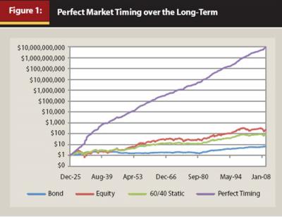
An initial $1 investment would grow to $6 (in real terms) over the test period if invested in bonds (which is a 2.2 percent annualized geometric real return), $75 in the balanced 60/40 portfolio that is rebalanced monthly (5.3 percent annualized geometric real return), $215 in equity (6.6 percent annualized geometric real return), and almost $10 billion if invested in the perfect market-timing portfolio (31.5 percent annualized geometric real return). The possibility of realizing results similar to the perfect market-timing portfolio in Figure 1 is why tactical strategies are so attractive. To put the likelihood of achieving perfect market timing in perspective, though, the probability of correctly guessing the asset class with the higher return for each month in the 1,008-month test-period would be materially less than one in a trillion (assuming the investor’s decision-making process was equivalent to a coin flip each year).
The Asset Allocation Decision
The relative importance of asset allocation has been well documented. In Brinson, Hood, and Beebower’s 1986 research paper “Determinants of Portfolio Performance” (perhaps the most well-known paper on asset allocation), the authors conclude that a portfolio’s asset allocation, or policy return, explained 93.6 percent of the variation in the 91 large U.S. pension plans tested. Brinson, Singer, and Beebower (1991) confirmed the results in the original paper, but found a slightly lower number, 91.5 percent. Additional research has confirmed these general findings (Ibbotson and Kaplan 2000; Tokat et al. 2006). Given the importance of the asset allocation decision, the ability to correctly shift among asset classes would seem to hold great promise; unfortunately, academic research on the market-timing abilities of mutual funds and portfolio managers has generally not been favorable.
In a paper titled “Likely Gains from Market Timing” by Sharpe (1975), the author uses algebraic tests seeking to quantify the likely benefits from market timing, and notes, “Unless a manager can predict whether the market will be good or bad each year with considerable accuracy (e.g., be right at least 7 times out of 10), he should probably avoid attempts to time the market altogether.” Sharpe also notes, “It is said that the military is usually well-prepared to fight the previous war.… Unfortunately for the military, the next war may differ from the last one. And unfortunately for investors, the next market may also differ from the last one.”
Using annual returns for 57 open-end mutual funds, Treynor and Mazuy (1966) developed a test of market timing and found significant ability in only 1 fund out of 57 in their sample. Their process, known as the “Treynor-Mazuy model” (TM Model), has become a widely used measure to analyze the timing ability of mutual funds. Research based on this test by Henriksson (1984), Grinblatt and Titman (1988), and Connor and Korajczyk (1991), among others, have found that the majority of portfolio managers are not able to successfully make market-timing decisions.
The Risk Dynamic
In order to determine the additional risk associated with tactical investing, an analysis was conducted. The analysis assumes that similar to the test conducted for Figure 1, an investor selects between one of two portfolios (or asset classes) annually. The first portfolio is an equity portfolio, which has an assumed return of 12 percent with an annual standard deviation of 22 percent—approximately equal to the arithmetic return and standard deviation of the S&P 500 from January 1926 to December 2009, at 11.82 percent and 22.15 percent, respectively. The second portfolio is a bond portfolio, which has an assumed nominal rate of return of 5 percent and an annual standard deviation of 4 percent—approximately equal to the arithmetic return and standard deviation of the Ibbotson Intermediate Government Bond Index from January 1926 to December 2009, at 5.34 percent and 4.22 percent, respectively.
For simplicity purposes with respect to the calculations, the correlation between the two portfolios is assumed to be zero, while the actual correlation of the two portfolios during the test period was .09. Approximations were selected for the analysis versus using actual historical data for a variety of reasons, primarily to enable the author to generate significantly more test periods than historical data are available for, as well as to allow the analysis to be more easily replicated by the reader.
The risk-free rate for Sharpe ratio calculations is assumed to be 3 percent, and the minimum acceptable return (MAR) for downside deviation and Sortino ratio calculations is assumed to be 0 percent (any negative return would be considered risky). The Sharpe ratio is calculated by subtracting the risk-free return from the geometric return of the portfolio and dividing it by the standard deviation. This gives a “risk-adjusted” measure of the portfolio return. The Sortino ratio is similar to the Sharpe ratio but is based on downside risk versus standard deviation. Downside risk is calculated by comparing the return of the investment to its MAR, whereby only the returns below the MAR are considered risky.
While this analysis assumes the entire portfolio is moved between bond and equity, it is unlikely most advisers will implement such a dramatic strategy. Instead, an adviser would only be likely to tactically reallocate the portfolio within a given range; for example, a portfolio with a 50 percent target equity allocation could be no more than 70 percent and no less than 30 percent equities. For this type of tactical investing, this analysis provides guidance on the additional risk associated with whatever degree tactical allocation is being implemented within a portfolio. Using the previous example, the tactical range for the portfolio would be 40 percent of the portfolio, because the portfolio will have no less than 30 percent bonds and no more than 70 percent cash/fixed. Therefore, this analysis provides guidance on the risk associated with tactically reallocating 40 percent of the portfolio; the remaining 60 percent is essentially a static allocation.
The analysis is based on moving between bonds and equities because the equity allocation of the portfolio is the primary determinant of its risk (note previous text on the importance of asset allocation). However, this line of research can just as easily be applied to more subtle changes to portfolios, such as comparing the impact of using bonds and real estate, bonds and commodities, equities and cash, etc. As long as you are dynamically moving between two (or more) asset classes that provide some diversification benefit from holding them together, making changes to the allocation can (and will) have significant implications for the risk of the portfolio.
The simulator for the analysis was built in Microsoft Excel by the author. The probability of correctly selecting the higher return is randomly generated for each run of each year using the Rand function, which randomly populates a value between 0 and 1. If the value generated by the Rand function is less than or equal to the probability of being correct, it is assumed the investor selects the portfolio that yields the higher return (is correct) and vice versa. All tests are based on a 10,000 run (10,000 year) simulation.
Results
Table 1 includes various statistics for a variety of probabilities of correctly selecting next year’s higher performing asset class, as well as a 50/50 balanced portfolio and the bond and equity portfolios. It is worth noting that an investor who is correct 0 percent of the time would have an average equity allocation during the entire test period of approximately 39 percent, while an investor who is right 100 percent of the time would have an average equity allocation of approximately 62 percent. The investor who is correct more often has a higher average allocation to equities because equities had a higher expected return than bonds (on average).
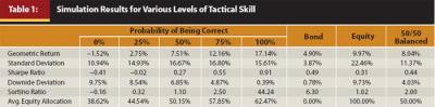
There are a variety of key takeaways from Table 1. First, the 50 percent correct portfolio, which is the portfolio in which it is assumed the investor correctly guessed the portfolio with the higher return 50 percent of the time, had a lower return, higher standard deviation, and higher downside risk (downside deviation) when compared to the 50/50 balanced portfolio. This means the average investor, who is correct 50 percent of the time when making tactical allocation decisions, has clearly implemented a suboptimal strategy for his or her portfolio on a return, risk, and risk-adjusted basis when compared to a pure static asset allocation strategy.
It may surprise the reader that the 50 percent correct portfolio had an approximately 50 percent allocation to equities. Intuitively, the reader might think that equities should be used more frequently than bonds because equities had a higher return approximately 62 percent of the time. However, while the probability of selecting equities is higher when the person is correct, the probability of selecting bonds is higher when the person is wrong, and these offset when someone is only 50 percent correct. The more often someone is correct, though, the more likely they are to have a higher equity allocation, as equities had a higher average return than bonds. This concept is relayed visually in Table 2.
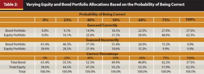
Table 2 shows how often one of the four possible outcomes occurred: being correct and selecting bonds, being correct and selecting equities, being incorrect and selecting bonds, and being incorrect and selecting equities. Because equities have a higher return than bonds, the probability of correctly selecting equities increases the more someone is correct. Therefore, again, this study is in no way biasing the results toward equities or a portfolio with a higher assumed return than a static portfolio.
Due to the nature of the “skilled” strategy (dynamically moving between bonds and equities), standard deviation may not be the most appropriate method to define portfolio risk. For example, the 100 percent correct portfolio has approximately the same standard deviation as the 25 percent correct portfolio, yet it has virtually no downside risk (as defined by the downside deviation). This point can be seen more clearly in Figure 2, which includes the distribution of annual returns for the 50/50 static portfolio, the 50 percent correct portfolio, and the 100 percent correct portfolio. Given the non-normal return distributions, statistics such as downside risk and the Sortino ratio are likely better proxies for risk and risk-adjusted return.
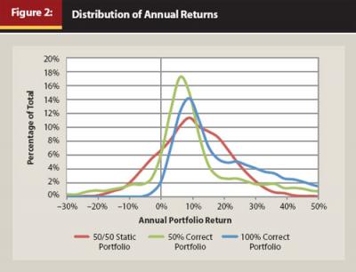
It should not surprise the reader that the return distribution for the 100 percent correct portfolio is incredibly favorable, with very little downside risk and a high degree of positive skewness (a “right tail” in the distribution). In Table 1, the 100 percent correct and bond portfolios have similar downside risk statistics because the probability of either being negative is small. For additional information on downside risk approaches to investing, see Swisher and Kasten (2005) or Sortino and Satchell (2001).
When equalizing the lifetime equity exposure (as you are correct more often you tend to have a higher total allocation to equities), you would need to be correct 65 percent of the time to get an equivalent Sharpe ratio for a static allocation strategy (which would be a 54 percent static equity allocation portfolio) and 66 percent of the time to get an equivalent Sortino ratio for a static allocation strategy (which would be a 55 percent static equity allocation). This point is worth repeating: in order to replicate the risk-adjusted return associated with a static allocation approach assuming the same equity allocation, you need to be correct approximately 66 percent (two-thirds) of the time when making tactical allocation decisions. These results are similar to those of Sharpe (1975), discussed previously. For those investors not concerned with risk, you would only need to be correct approximately 54 percent of the time to achieve the same return as a static allocation approach. However, such an investor would be subjected to materially more risk (defined as either standard deviation or downside risk), which is in contrast to the fundamental goal of most tactical strategies.
Tax Implications
While the potential tax implications of tactical reallocating are not going to be of concern in a tax-free or tax-deferred investment portfolio (IRA, 401(k), pension, or endowment), the additional trading associated with tactical reallocation can have a material effect on the long-term after-tax returns realized by an investor in a taxable portfolio. There are two types of capital gains realized by investors in the securities markets: short-term and long-term. Short-term capital gains, or gains on those investments held a year or less, are taxed at the taxpayer’s ordinary (or marginal) tax rate, which is currently as high as 35 percent. The U.S. tax code has historically provided certain tax benefits for long-term capital gains, or gains on those investments held more than a year, which are typically taxed at a lower rate. The long-term capital gains rate is currently 15 percent or 5 percent for individuals in the lowest two marginal income tax brackets, although these rates could easily have changed by the time this paper is published given the current uncertainty surrounding future tax policy.
The tax inefficiency of tactically reallocating a portfolio depends largely on the frequency of trading. If changes are made to the allocation only every few years, then the difference in the after-tax returns of static and dynamic strategies would not be material (assuming an equalized equity allocation and ignoring risk). However, an approach in which the allocation is updated more frequently, say every six months, would incur additional “costs” because of the higher short-term capital gains tax rate, as well as the consequent impact on compounding (assuming the taxes are paid from that same account).
While simple formulas can be used to determine the different growth rates for investments with varying levels of tax efficiency, the actual implementation in portfolios involves costs that are incredibly difficult (if not impossible) to model on a pure algebraic basis. Therefore, in order to determine the tax costs associated with tactically reallocating a portfolio, a simulator like the one used for the first analysis in this paper was created. For this analysis, two types of portfolios are tested. The first is a static portfolio, in which the allocation is rebalanced annually to bring the allocation (between bonds and equities) back to the target allocation. It is assumed that all gains from the bond portion are realized annually at short-term capital gains rates. The equity portion is assumed to grow over time, and all gains are taxed at the long-term capital gains rate, which is assumed to be 15 percent (and constant) for the analysis.
All taxes are assumed to be paid from the account at the end of the year, reducing the account balance. Any losses are treated as a “credit,” effectively increasing the account balance. The implicit assumption with the credit methodology is that there is other investment income from another taxable portfolio that can “soak up” these losses and that this portfolio effectively receives the benefit of the taxes that would have been paid from the gains from the other account. The cost basis for the equity account is tracked over time, and it is assumed that at the end of the test period the equity account is liquidated and the capital gains tax is paid based on the appreciation. Taxes are paid annually on the bond piece, therefore an end-of-period liquidation for tax purposes is not necessary, apart from the last year.
The second portfolio is the tactical portfolio, in which the allocation changes annually based on a “guess” as to which asset class, bond or equity, will have the higher return the following year. If the portfolio is invested entirely in the bond piece the entire gain is considered to be short-term and is realized at the end of the year. If the equity piece is only held for a year (such that the portfolio is bond in year one, equity in year two, and then back to bond in year three) the gains (losses) in the equity account are taxed (credited) at short-term capital rates. If the equity piece is held for more than one year the gains are taxed at long-term rates. Note, the bond piece can also have losses resulting in credit, although it is unlikely. Unlike the static portfolio, which incurs taxes annually from rebalancing the portfolio back to its target allocation, the tactical portfolio only incurs taxes if it is invested in bonds or if it sells out of equities for the year. In different simulations there are often long periods (such as 5+ years) when the equity account in the tactical portfolio grows without the burden of paying taxes, and then long-term capital gains are paid based on the total appreciation during the period.
If an investor were able to correctly select the asset class (bond or equity) that is going to outperform over the following year, he or she would have to correctly select the future outperforming asset 54 percent of the time to achieve the same return as a 50/50 static allocation. Therefore, in order to determine the tax cost of tactical reallocation, the after-tax performance of a tactical investor who is correct 54 percent of the time is compared to a 50/50 static allocation. Note, in the absence of taxes, the expected return for the portfolios would be the same, so any difference would be a result of differing tax payments between the two portfolios.
For the analysis, both portfolios experienced the same annual returns for bond and equity portions (although they will have different total portfolio returns based on their actual investments). Each simulation compares the return over a 1,000-year period, and 1,000 runs are considered for each scenario. While an investor may consider a 1,000-year investment period unreasonable, the longer the holding period, the more the difference between the two return series is caused by different tax structures and less by random chance.
The long-term capital gains rate for the analysis is assumed to be 15 percent and the short-term capital gains rates are tested between 15 percent and 45 percent in 1 percent increments. While capital gains rates may change (the highest current short-term capital gains rate is 35 percent, but 45 percent was the highest rate tested), the key to the analysis is the difference, or spread, between the two rates, which is currently 20 percent. The results are included in Figure 3.

As the reader can see from Figure 3, even if the short-term capital gains rate and the long-term capital gains rate are the same (15 percent), the expected return of the tactical allocation strategy is approximately 40 basis points (bps) lower than the static approach. This can be attributed to the reduced compounding from realizing gains on a more frequent basis. If the short-term capital gains rate is the current maximum rate of 35 percent (for a spread of 20 percent between the short-term and long-term rates) the long-term costs associated with tactical reallocation increase to approximately 77 bps per year. The slope of the linear regression suggests that the returns of the tactical strategy decrease by approximately 1 bp for each 1 percent difference in the tax rates with an intercept of –36 bps.
To give the reader an idea of the taxes paid by the tactical portfolio for the analysis, the probability of incurring short-term capital gains (on an annual basis) decreases from 66 percent if you’re correct 40 percent of the time, to 58 percent if you’re correct 70 percent of the time. The tactical portfolios also pay roughly twice the total taxes in relation to total account dollars on an annual basis as the static portfolios.
Given the after-tax performance reduction between 50 bps and 90 bps for the current range of short-term tax rates, how often does a tactical investor need to be correct in order to overcome the additional tax costs associated with tactical investing? Table 3 includes the after-tax outperformance of various tactical portfolios based on different short-term tax rates and probabilities of correctly selecting the higher performing asset, between bond and equity.
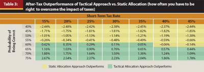
Based on the information in Table 2, an investor would need to be correct approximately 58 percent of the time in order to overcome the tax costs associated with a tactical allocation approach to achieve the same portfolio return as a static allocation. This is a 4 percent increase over the same figure when taxes are not considered. On a risk-adjusted basis taking into account the expected performance difference for various short-term capital gains rates, in order to achieve an equivalent Sharpe ratio as a portfolio with the same expected equity allocation, an investor would need to be correct approximately 69 percent of the time; to have an equivalent Sortino ratio an investor would need to be correct approximately 70 percent of the time.
Additional Tactical Considerations
The two tests conducted thus far have been concerned primarily with costs associated with tactical trading that can be quantified for investors of all sizes. There are additional costs, though, such as the cost of benchmark variation, the difficulty of identifying luck and skill, and the trading expenses incurred with tactical reallocation that need to be considered when determining whether or not to use a tactical strategy. Each of these represents a “cost” associated with a tactical strategy that makes it more difficult to implement.
“Benchmark variation” is a significant issue for advisers and investors, because a successful tactical asset allocation is fundamentally a contrarian strategy. A successful tactical allocator needs to make decisions that are contrary to what the market is doing, and often requires a long-term perspective. Julian Roberstson proved correct in his assessment that tech stocks were overpriced when the bubble burst, but his Tiger Management hedge fund, with assets that peaked at $22 billion in 1998, was forced to close just before the crash in March 2000. As John Maynard Keynes noted, “The market can stay irrational longer than you can stay solvent.”
Differentiating between luck and skill is incredibly difficult in the investment industry. Clients are not usually patient enough to allow a manager time to generate a track record that a statistician would reasonably consider to be statistically significant (five years at the absolute minimum), yet clients still need to be able to hold the manager accountable for his or her performance, and make changes accordingly. Cornell (2008) noted, “The problem is that skill and luck are not independently observable. Instead, all that can be observed is their combined impact, which is here called performance. The central question, therefore, is to determine how much can be learned about skill by observing performance.”
The more often an investor trades, the higher the costs incurred by the investor. These costs come in a variety of shapes and sizes, such as commissions, bid/ask spreads, and market impact. Larger investors tend to pay lower explicit trading costs (such as commissions) than smaller investors, but they also tend to pay higher implicit costs (such as market impact). More frequent trading models are going to incur more costs and therefore require a higher level of certainty to ensure their success. While a $10 trading commission and bid/ask spread of .05 percent may not seem material in light of the potential benefits from a tactical strategy, every trade reduces an investor’s wealth and reduces the attractiveness of a tactical asset allocation strategy.
Conclusion
The research conducted for this paper suggests that a long-term static allocation strategy is likely to produce higher risk-adjusted performance than a tactical asset allocation approach. In order to achieve the same risk-adjusted performance as a static portfolio with the same equity allocation, you must be able to correctly select the outperforming asset class (either bond or equity) roughly 66 percent of the time. In order to achieve the same risk-adjusted performance on an after-tax basis as a static portfolio with the same equity allocation, you must be able to correctly select the outperforming asset class roughly 70 percent of the time. These results are similar to the past findings of Sharpe (1975), who notes a portfolio manager should be right at least 7 times out of 10 before engaging in market timing.
The likelihood of a tactical asset allocation outperforming a static allocation decreases further when considering the additional costs incurred by tactical investors, such as benchmark deviation, the difficulty of differentiating between luck and skill, and the additional trading expenses. In summary, despite the appeal of a tactical asset allocation approach, a static asset allocation is likely to lead to a higher risk-adjusted performance for the vast majority of investors.
References
Brinson, Gary P. , L. Randolph Hood, and Gilbert L. Beebower. 1986. “Determinants of Portfolio Performance.” Financial Analysts Journal 42, 4 (July/August): 39–44.
Brinson, Gary P., Brian D. Singer, and Gilbert L. Beebower. 1991. “Determinants of Portfolio Performance II: An Update.” Financial Analysts Journal 47, 3 (May/June): 40–48.
Connor, G. and R. Korajczyk. 1991. “The Attributes, Behavior, and Performance of U.S. Mutual Funds.” Review of Quantitative Finance and Accounting 1: 5–26.
Cornell, Bradford. 2008. “Luck, Skill, and Investment Performance.” Working Paper: www.hss.caltech.edu/~bcornell/PUBLICATIONS/2008%20Cornell-Luck%20Skill.pdf.
Grinblatt, M. and S. Titman. 1988. “The Evaluation of Mutual Fund Performance: An Analysis of Monthly Returns.” Working Paper, University of California, Los Angeles.
Henriksson, Roy D. 1984. “Market Timing and Mutual Fund Performance: An Empirical Investigation.” The Journal of Business 57, 1 (January): 73–96.
Ibbotson, Roger G. and Paul D. Kaplan. 2000. “Does Asset Allocation Policy Explain 40, 90, or 100 Percent of Performance?” Financial Analysts Journal 56, 1: 26–33.
Sharpe, William. 1975. “Likely Gains from Market Timing.” Financial Analysts Journal 31, 2 (March/April): 60–69.
Sortino, Frank and Stephen Satchell. 2001. Managing Downside Risk in Financial Markets. Butterworth-Heinemann.
Swisher, Pete K. and Gregory W. Kasten. 2005. “Post-Modern Portfolio Theory.” Journal of Financial Planning 18, 9 (September): 74–66.
Tokat, Yesim, Nelson W. Wicas, and Francis M. Kinniry. 2006. “The Asset Allocation Debate: A Review and Reconciliation.” Journal of Financial Planning 19, 10 (October): 52–61
Treynor, J. and K. Mazuy. 1966. “Can Mutual Funds Outguess the Market?” Harvard Business Review 43 (July/August): 131–136.